Corner Proposal Network for Anchor-free, Two-stage Object Detection

1. 动机

   • anchor-free
   • two-stage
     • 先找potential corner keypoints
     • classify each proposal
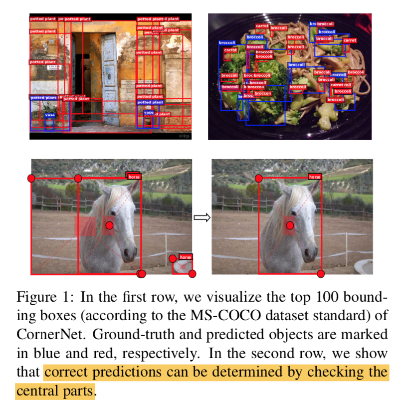
   • corner-based方法：对于objects of various scales有效，在训练中避免产生过多的冗余false-positive proposals，但是在结果上会出现更多的fp
   • 得到的是competitive results

2. 论点

   • anchor-based methods对形状奇怪的目标容易漏检

   • anchor-free methods容易引入假阳caused by mistakely grouping

     • thus an individual classifier is strongly required

   • Corner Proposal Network (CPN)

     • use key-point detection in CornerNet
     • 但是group阶段不再用embedding distance衡量，而是用a binary classifier
     • 然后是multi-class classifier，operate on the survived objects
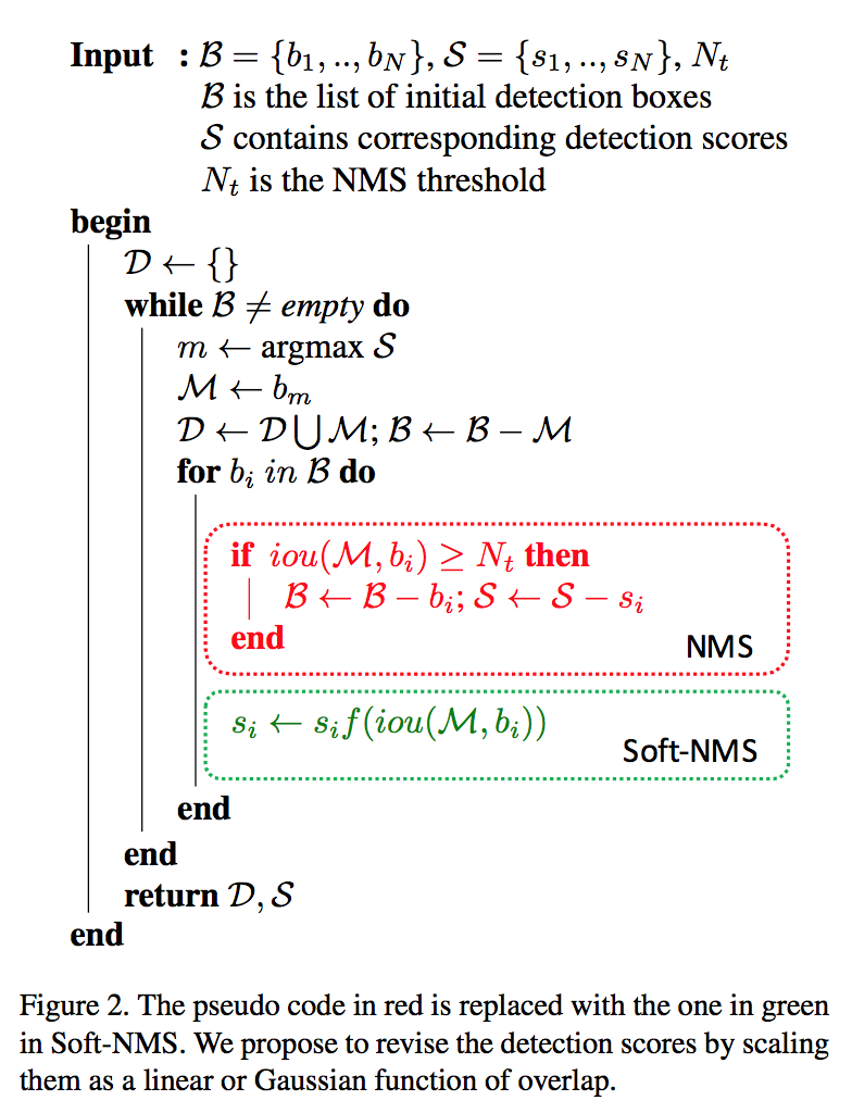
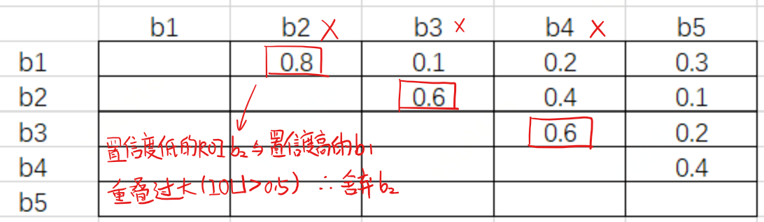
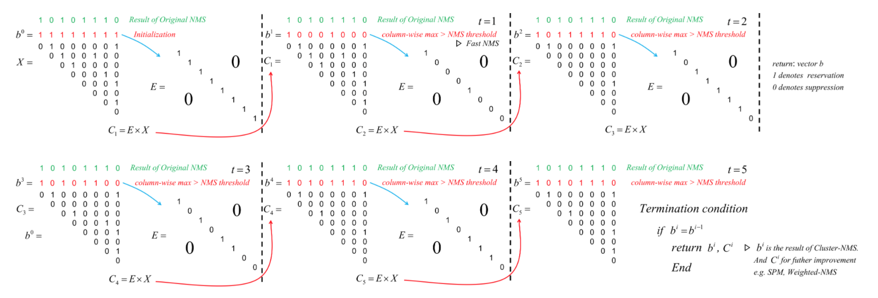
     • 最后soft-NMS

RefineNet: Multi-Path Refinement Networks for High-Resolution Semantic Segmentation

引用量1452，但是没有几篇技术博客？？

1. 动机

   • 语义分割
     • dense classification on every single pixel
   • refineNet
     • long-range residual connections
     • chained residual pooling

2. 论点

   • pooling/conv stride：
     • losing finer image structure
     • deconv is not able to recover the lost info
   • atrous
     • high reso：large computation
     • dilated conv：coarse sub-sampling of feature
   • FCN
     • fuse features from all levels
     • stage-wise rather than end-to-end???存疑

   • this paper

     • main idea：effectively exploit middle layer features
     • RefineNet
       • fuse all level feature
       • residual connections with identity skip
       • chained residual pooling to capture background context：看描述感觉像inception downsamp
       • end-to-end
       • 是整个分割网络中的一个component

     

3. 方法

   

   • backbone
     • pretrained resnet
     • 4 blocks：x4 - x32，each block：pool-residual
     • connection：每个输出连接一个RefineNet unit
   • 4-cascaded architecture
     • final ouput：
       • high-resolution feature maps
       • dense soft-max
       • bilinear interpolation to origin resolution
     • cascade inputs
       • output from backbone block
       • ouput from previous refineNet block
   • refineNet block
     • adapt conv：
       • to adapt the dimensionality and refine special task
       • BN layers are removed
       • channel 512 for R4，channel 256 for the rest
     • fusion：
       • 先用conv to adapt dimension and recale the paths
       • 然后upsamp
       • summation
       • 如果single input：walk through and stay unchanged
     • chained residual pooling：
       • aims to capture background context from a large image region
       • chained：efficiently pool features with multiple window sizes
       • pooling blocks：s1 maxpooling+conv
       • in practice用了两个pooling blocks
       • use one ReLU in the chained residual pooling block
     • output conv：
       • 一个residual：to employ non-linearity
       • dimension remains unchanged
       • final level：two additional RCUs before the final softmax prediction
   • residual identity mappings
     • a clean information path not block by any non-linearity：所有relu都在residual path里面
     • 只有chained residual pooling模块起始时候有个ReLU：one single ReLU in each RefineNet block does not noticeably reduce the effectiveness of gradient flow
     • linear operations：
       • within the fusion block
       • dimension reduction operations
       • upsamp operations

4. 其他结构

   

   • 级联的就叫cascaded
   • 一个block就叫single
   • 多个input resolution就叫mult-scale

5. 实验

   • 4-cascaded works better than 1-cas & 2-cas
   • 2-scale works better than 1-scale

[papers]

• [centerNet] 真centerNet: Objects as Points，utexas，这个是真的centerNet，基于分割架构，预测中心点的heatmap，以及2-N个channel其他相关参数的回归

• [cornet-centerNet] centerNet: Keypoint Triplets for Object Detection，这个抢先叫了centerNet，但是我觉得叫corner-centerNet更合适，它是基于cornerNet衍生的，在cornerNet的基础上再加一刀判定，基于角点pair的中心点是否是前景来决定是否保留这个框

• [centerNet2] Probabilistic two-stage detection，utexas，

centerNet: Objects as Points

1. 动机

   • anchor-based

     • exhaustive list of potential locations
     • wasteful, inefficient, requires additional post-processing

   • our detector

     • center：use keypoint estimation to find center points
     • other properties：regress

   • tasks

     • object detection
     • 3d object detection

     • multi-person human pose estimation

       

2. 论点

   • 相比较于传统一阶段、二阶段检测
     • anchor：
       • box & kp：一个是框，一个是击中格子
       • nms：take local peaks，no need of nms
       • larger resolution：hourglass架构，输出x4的heatmap，eliminates the need for multiple anchors
   • 相比较于key point estimantion network
     • them：require grouping stage
     • our：只定位一个center point，no need for group or post-processing

3. 方法

   • loss

     • 关键点loss

       • center point关键点定义：每个目标的gt point只有一个，以它为中心，做object size-adaptive的高斯penalty reduction，overlap的地方取max

       • focal loss：基本与cornetNet一致

         $$L_k = \frac{-1}{N}\sum_{x,y,c} \begin{cases} (1-\hat Y)^\alpha log(\hat Y), if Y=1\\ (1-Y)^\beta \hat Y^\alpha log(1-\hat Y), otherwise \end{cases}$$
         • $\alpha=2, \beta=4$
         • background points有penalty，根据gt的高斯衰减来的

     • offset loss

       • 只有两个通道(x_offset & y_offset)：shared among categories
       • gt的offset是原始resolution/output stride向下取整得到
       • L1 loss

   • centerNet

     • output

       • 第一个部分：中心点，[h,w,c]，binary mask for each category
       • 第二个部分：offset，[h,w,2]，shared among
       • 第三个部分：size，[h,w,2]，shared among
         • L1 loss，use raw pixel coordinates
       • overall
         • C+4 channels，跟传统检测的formulation是一致的，只不过传统检测gt是基于anchor计算的相对值，本文直接回归绝对值
         • $L_{det} = L_k + \lambda_{size} L_{size} + \lambda_{off} L_{off}$
         • 其他task的formulation看第一张图

     • inference workflow

       • local peaks：
         • for each category channel
         • all responses greater or equal to its 8-connected neighbors：3x3 max pooling
         • keep the top100
       • generate bounding boxes
         • 组合offset & size predictions
         • ？？？？没有后处理了？？？假阳？？？？

     • encoder-decoder backbone：x4

       • hourglass104
         • stem：x4
         • modules：两个
       • resnet18/101+deformable conv upsampling
         • 3x3 deformable conv, 256/128/64
         • bilinear interpolation

       • DLA34+deformable conv upsampling

         

     • heads

       • independent heads
       • one 3x3 conv，256
       • 1x1 conv for prediction

4. 总结

   个人感觉，centerNet和anchor-based的formulation其实是一样的，

   • center的回归对标confidence的回归，区别在于高斯/[0,1]/[0,-1,1]
   • size的回归变成了raw pixel，不再基于anchor
   • hourglass结构就是fpn，级联的hourglass可以对标bi-fpn
   • 多尺度变成了单一大resolution特征图，也可以用多尺度预测，需要加NMS

centerNet2: Probabilistic two-stage detection

1. 动机

   • two-stage
   • probabilistic interpretation
   • the suggested pipeline
     • stage1：infer proper object-backgroud likelihood，专注前背景分离
     • stage2：inform the overall score
   • verified on COCO
     • faster and more accurate than both one and two stage detectors
     • outperform yolov4
     • extreme large model：56.4 mAP
     • standard ResNeXt- 32x8d-101-DCN back：50.2 mAP

2. 论点

   • one-stage detectors
     • dense predict
     • jointly predict class & location
     • anchor-based：RetinaNet用focal loss来deal with 前背景imbalance
     • anchor-free：FCOS & CenterNet不基于anchor基于grid，缓解imbalance
     • deformable conv：AlignDet在output前面加一层deformable conv to get richer features
     • sound probablilistic interpretation
     • heavier separate classification and regression branches than two-stage models：如果类别特别多的情况，头会非常重，严重影响性能
     • misaligned issue：一阶段预测是基于local feature，感受野、anchor settings都会影响与目标的对齐程度
   • two-stage detectors
     • first RPN generates coarse object proposals
     • then per-region head to classify and refine
     • ROI heads：Faster-RCNN用了两个fc层作为ROI heads
     • cascaded：CascadeRCNN用了三个连续的Faster-RCNN，with a different positive threshold
     • semantic branch：HTC用了额外的分割分支enhance the inter-stage feature flow
     • decouple：TSD将cls&pos两个ROI heads解耦
     • weak RPN：因为尽可能提升召回率，proposal score也不准，丧失了一个clear的probabilistic interpretation
     • independent probabilistic interpretation：两个阶段各训各的，最后的cls score仅用第二阶段的
     • slow：proposals太多了所以slow down
   • other detectors
     • point-based：cornetNet预测&组合两个角点，centerNet预测中心点并基于它回归长宽
     • transformer：DETR直接预测a set of bounding boxes，而不是传统的结构化的dense output

   • 网络结构

     • one/two-stage detectors：image classification network + lightweight upsampling layers + heads
     • point-based：FCN，有symmetric downsampling and upsampling layer，预测一个小stride的heatmap
     • DETR：feature extraction + transformer decoder

   • our method

     

     • 第一个阶段
       • 做二分类的one-stage detector，提前景，
       • 实现上就用region-level feature+classifier（FCN-based）
     • 第二阶段
       • 做position-based类别预测
       • 实现上既可以用一个Faster-RCNN，也可以用classifier
     • 最终的loss由两个阶段合并得到，而不是分阶段训练
     • 跟former two-stage framework的主要不同是
       • 加了joint probabilistic objective over both stages
       • 以前的二阶段RPN的用途主要是最大化recall，does not produce accurate likelihoods
     • faster and more accurate
       • 首先是第一个阶段的proposal更少更准
       • 其次是第二个阶段makes full use of years of progress in two-stage detection，二阶段的设计站在伟人的肩膀上

3. 方法

   • joint class distribution：先介绍怎么将一二阶段联动
     • 【第一阶段的前背景score】 乘上 【第二阶段的class score】
     • $P(C_k) = \sum_o P(C_k|O_k=o)P(O_k=o)$
     • maximum likelihood estimation
       • for annotated objects
         • 退阶成independent maximum-likelihood
         • $log P(C_k) = log P(C_k|O_k=1) + log P(O_k=1)$
       • for background class
         • 不分解
         • $log P(bg) = log( P(bg|O_k=1) * P(O_k=1) + P(O_k=0))$
         • lower bounds，基于jensen不等式得到两个不等式
         • $log P(bg) \ge P(O_k=1) * log( P(bg|O_k=1))$：如果一阶段前景率贼大，那么就
         • $log P(bg) \ge P(O_k=0)$：
         • optimize both bounds jointly works better

   • network design：介绍怎么在one-stage detector的基础上改造出一个two-stage probabilistic detector

     • experiment with 4 different designs for first-stage RPN
     • RetinaNet
       • RetinaNet其实和two-stage的RPN高度相似核心区别在于：
         • a heavier head design：4-conv vs 1-conv
           • RetinaNet是backbone+fpn+individual heads
           • RPN是backbone+fpn+shared convs+individual heads
         • a stricter positive and negative anchor definition：都是IoU-based anchor selection，thresh不一样
         • focal loss
       • first-stage design
         • 以上三点都在probabilistic model里面保留
         • 然后将separated heads改成shared heads
     • centerNet
       • 模型升级
         • 升级成multi-scale：use ResNet-FPN back，P3-P7
         • 头是FCOS那种头：individual heads，不share conv，然后cls branch预测centerness+cls，reg branch预测regress params
         • 正样本也是按照FCOS策略：position & scale-based
       • 升级模型进行one-stage & two-stage实验：centerNet*
     • ATSS
       • 是一个adaptive IoU thresh的方法，centerness来表示一个格子的score
       • 我们将centerness*classification score定义为这个模型的proposal score
       • 另外就是two-stage下还是将RPN的cls & reg heads合并
     • GFL：还没看过，先跳过吧
     • second-stage designs：FasterRCNN & CascadeR- CNN
     • deformable conv：这个在centerNetv1的ResNet和DLA back里面都用了，在v2里面，主要是用ResNeXt-32x8d-101-DCN，

   • hyperparameters for two-stage probabilistic model

     • 两阶段模型通常是用P2-P6，一阶段通常用P3-P7：我们用P3-P7
     • increase the positive IoU threshold：0.5 to [0.6,0.7,0.8]
     • maximum of 256 proposals （对比origin的1k）
     • increase nms threshold from 0.5 to 0.7
     • SGD，90K iterations
     • base learning rate：0.02 for two-stage & 0.01 for one-stage，0.1 decay
     • multi-scale training：短边[640,800]，长边不超过1333
     • fix-scale testing：短边用800，长边不超过1333
     • first stage loss weight：0.5，因为one-stage detector通常用0.01 lr开始训练

4. 实验

   • 4种design的对比

     • 所有的probabilistic model都比one-stage model强，甚至还快（因为简化了脑袋）
     • 所有的probabilistic FasterRCNN都比原始的RPN-based FasterRCNN强，也快（因为P3-P7比P2-P6的计算量小一半，而且第二阶段fewer proposals）

     • CascadeRCNN-CenterNet design performs the best：所以以后就把它叫CenterNet2

       

   • 和其他real-time models对比

     • 大多是real-time models都是一阶段模型

     • 可以看到二阶段不仅能够比一阶段模型还快，精度还更高

       

   • SOTA对比

     • 报了一个56.4%的sota，但是大家口碑上好像效果很差
     • 不放图了

corner-centerNet: Keypoint Triplets for Object Detection

1. 动机

   • based on cornerNet

   • triplet

     • corner keypoints：weak grouping ability cause false positives

     • correct predictions can be determined by checking the central parts

       

   • cascade corner pooling and center poolling

2. 论点

   • whats new in CenterNet
     • triplet inference workflow
       • after a proposal is generated as a pair of corner keypoints
       • checking if there is a center keypoint of the same class
     • center pooling
       • for predicting center keypoints
       • by making the center keypoints on feature map having the max sum Hori+Verti responses
     • cascade corner pooling
       • equips the original corner pooling module with the ability of perceiving internal information
       • not only consider the boundary but also the internal directions
   • CornetNet痛点
     • fp rate高
     • small object的fp rate尤其高
     • 一个idea：cornerNet based RPN
       • 但是原生RPN都是复用的
       • 计算效率？

3. 方法

   • center pooling

     • geometric centers & semantic centers

     • center pooling能够有效地将语义信息最丰富的点（semantic centers）传达到物理中心点（geometric centers），也就是central region

       

MegDet: A Large Mini-Batch Object Detector

1. 动机

   • past methods mainly come from novel framework or loss design

   • this paper studies the mini-batch size

     • enable training with a large mini-batch size
     • warmup learning rate policy
     • cross-gpu batch normalization

   • faster & better acc

2. 论点

   • potential drawbacks with small mini-batch sizes

     • long training time

     • inaccurate statistics for BN：previous methods use fixed statistics from ImageNet which is a sub-optimal trade-off

     • positive & negative training examples are more likely imblanced

     • 加大batch size以后，正负样本比例有提升，所以yolov3会先锁着back开大batchsize做warmup

       

   • learning rate dilemma

     • large min-batch size usually requires large learning rate
     • large learning rate is likely leading to convergence failure
     • a smaller learning rate often obtains inferior results

   • solution of the paper

     • linear scaling rule
     • warmup
     • Cross-GPU Batch Normalization (CGBN)

3. 方法

   • warmup

     • set up the learning rate small enough at the be- ginning
     • then increase the learning rate with a constant speed after every iteration, until fixed

   • Cross-GPU Batch Normalization

     • 两次同步

     • tensorpack里面有

       

       

4. 一次同步

   • 异步BN：batch size 较小时，每张卡计算得到的统计量可能与整体数据样本具有较大差异

     

   • 同步：

   • 需要同步的是每张卡上计算的统计量，即BN层用到的均值$\mu$和方差$\sigma^2$

   • 这样多卡训练结果才与单卡训练效果相当

   • 两次同步：

   • 第一次同步均值：计算全局均值

   • 第二次同步方差：基于全局均值计算各自方差，再取平均

   • 一次同步：

     • 核心在于方差的计算

     • 首先均值：$\mu = \frac{1}{m} \sum_{i=1}^m x_i$

       • 然后是方差： $$\sigma^2 = \frac{1}{m} \sum_{i=1}^m (x_i-\mu)^2 = \frac{1}{m} \sum_{i=1}^m x_i^2 - \mu^2\\ =\frac{1}{m} \sum_{i=1}^m x_i^2 - (\frac{1}{m} \sum_{i=1}^m x_i)^2$$

  * 计算每张卡的$\sum x_i$和$\sum x_i^2$，就可以一次性算出总均值和总方差

RFB: Receptive Field Block Net for Accurate and Fast Object Detection

1. 动机

   • RF block：Receptive Fields
   • strengthen the lightweight features using a hand-crafted mechanism：轻量，特征表达能力强
   • assemble RFB to the top of SSD

2. 论点

   • lightweight

     • enhance feature representation

   • 人类

     • 群智感受野（pRF）的大小是其视网膜图中偏心率的函数
     • 感受野随着偏心率而增加
     • 更靠近中心的区域在识别物体时拥有更高的比重或作用

     • 大脑在对于小的空间变化不敏感

       

   • fixed sampling grid (conv)

     • probably induces some loss in the feature discriminability as well as robustness

   • inception

     • RFs of multiple sizes
     • but at the same center

   • ASPP

     • with different atrous rates
     • the resulting feature tends to be less distinctive

   • Deformable CNN

     • sampling grid is flexible

     • but all pixels in an RF contribute equally

       

   • RFB

     • varying kernel sizes
     • applies dilated convolution layers to control their eccentricities
     • 组合来模拟human visual system
     • concat

     • 1x1 conv for fusion

       

   • main contributions

     • RFB module: enhance deep features of lightweight CNN networks
     • RFB Net: gain on SSD
     • assemble on MobileNet

3. 方法

   • Receptive Field Block

     • 类似inception的multi-branch

     • dilated pooling or convolution layer

       

   • RFB Net

     • SSD-base

       

     • 头上有较大分辨率的特征图的conv层are replaced by the RFB module

     • 特别头上的conv层就保留了，因为their feature maps are too small to apply filters with large kernels like 5 × 5

       

     • stride2 module：每个conv stride2，那id path得变成1x1 conv？

PANet: Path Aggregation Network for Instance Segmentation

1. 动机

   • boost the information flow
   • bottom-up path
     • shorten information path
     • enhance accurate localization
   • adaptive feature pooling
     • aggregate all levels
     • avoiding arbitrarily assigned results
   • mask prediction head
     • fcn + fc
     • captures different views, possess complementary properties
   • subtle extra computational

2. 论点

   • previous skills: fcn, fpn, residual, dense
   • findings
     • 高层特征类别准，底层特征定位准，但是高层和底层特征之间的path太长了，不利于双高
     • past proposals make predictions based on one level
   • PANet
     • bottom-up path
       • shorten information path
       • enhance accurate localization
     • adaptive feature pooling
       • aggregate all levels
       • avoiding arbitrarily assigned results
     • mask prediction head
       • fcn + fc
       • captures different views, possess complementary properties

3. 方法

   • framework

     

     • b: bottom-up path
     • c: adaptive feature pooling
     • e: fusion mask branch

   • bottom-up path

     • fpn’s top-down path:
       • to propagate strong semantical information
       • to ensure reasonable classification capability
       • long path: red line, 100+ layers
     • bottom-up path:
       • enhances the localization capability
       • short path: green line, less than 10 layers

     • for each level $N_l$

       • input: $N_{l+1}$ & $P_l$
       • $N_{l+1}$ 3x3 conv & $P_l$ id path - add - 3x3 conv
       • channel 256
       • ReLU after conv

       

   • adaptive feature pooling

     • pool features from all levels, then fuse, then predict

     • steps

       • map each proposal to all feature levels
       • roi align
       • go through one layer of the following sub-networks independently
       • fusion operation (element-wise max or sum)

       • 例如，box branch是两个fc层，来自各个level的roi align之后的proposal features，先各自经过一个fc层，再share the following till the head，mask branch是4个conv层，来自各个level的roi align之后的proposal features，先各自经过一个conv层，再share the following till the head

         

     • fusion mask branch

       • fc layers are location sensitive
       • helpful to differentiate instances and recognize separate parts belonging to the same object
       • conv分支
         • 4个连续conv+1个deconv：3x3 conv，channel256，deconv factor=2
         • predict mask of each class：output channel n_classes
       • fc分支
         • from conv分支的conv3输出
         • 2个连续conv，channel256，channel128
         • fc，dim=28x28，特征图尺寸，用于前背景分类

       • final mask：add

         

4. 实验

   • heavier head
     • 4 consecutive 3x3 convs
     • shared among reg & cls
     • 在multi-task的情况下，对box的预测有效

CSPNET: A NEW BACKBONE THAT CAN ENHANCE LEARNING CAPABILITY OF CNN

1. 动机

   • propose a network from the respect of the variability of the gradients
   • reduces computations
   • superior accuracy while being lightweightening

2. 论点

   • CNN architectures design

     • ResNeXt：cardinality can be more effective than width and depth
     • DenseNet：reuse features
     • partial ResNet：high cardinality and sparse connection，the concept of gradient combination

   • introduce Cross Stage Partial Network (CSPNet)

     • strengthening learning ability of a CNN：sufficient accuracy while being lightweightening
     • removing computational bottlenecks：hoping evenly distribute the amount of computation at each layer in CNN

     • reducing memory costs：adopt cross-channel pooling during fpn

       

3. 方法

   • 结构

     • Partial Dense Block：节省一半计算
     • Partial Transition Layer：fusion last能够save computation同时精度不掉太多

     

     • 论文说fusion first使得大量梯度得到重用，computation cost is significantly dropped，fusion last会损失部分梯度重用，但是精度损失也比较小(0.1)。
     • it is obvious that if one can effectively reduce the repeated gradient information, the learning ability of a network will be greatly improved.

     

• Apply CSPNet to Other Architectures

  • 因为只有一半的channel参与resnet block的计算，所以无需再引入bottleneck结构了

  • 最后两个path的输出concat

    

• EFM

  

• fusion

    * 特征金字塔（FPN）：融合当前尺度和以前尺度的特征。
    * 全局融合模型（GFM）：融合所有尺度的特征。
    * 精确融合模型（EFM）：融合anchor尺寸上的特征。
  

  • EFM
    • assembles features from the three scales：当前尺度&相邻尺度
    • 同时又加了一组bottom-up的融合
    • Maxout technique对特征映射进行压缩

1. 结论

   从实验结果来看，

   • 分类问题中，使用CSPNet可以降低计算量，但是准确率提升很小；
   • 在目标检测问题中，使用CSPNet作为Backbone带来的提升比较大，可以有效增强CNN的学习能力，同时也降低了计算量。本文所提出的EFM比GFM慢2fps，但AP和AP50分别显著提高了2.1%和2.4%。

Non-maximum suppression：非极大值抑制算法，本质是搜索局部极大值，抑制非极大值元素

[nms]：standard nms，当目标比较密集、存在遮挡时，漏检率高

[soft nms]：改变nms的hard threshold，用较低的分数替代0，提升recall

[softer nms]：引入box position confidence，通过后处理提高定位精度

[DIoU nms]：采用DIoU的计算方式替换IoU，因为DIoU的计算考虑到了两框中心点位置的信息，效果更优

[fast nms]：YOLOACT引入矩阵三角化，会比Traditional NMS抑制更多的框，性能略微下降

[cluster nms]：CIoU提出，弥补Fast NMS的性能下降，运算效率比Fast NMS下降了一些

[mask nms]：mask iou计算有不可忽略的延迟，因此比box nms更耗时

[matrix nms]：SOLO将mask IoU并行化，比FAST-NMS还快，思路和FAST-NMS一样从上三角IoU矩阵出发，可能造成过多抑制。

[WBF]：加权框融合，Kaggle胸片异物比赛claim有用，速度慢，大概比标准NMS慢3倍，WBF实验中是在已经完成NMS的模型上进行的

1. nms
   • 过滤+迭代+遍历+消除
     • 首先过滤掉大量置信度较低的框，大于confidence thresh的box保留
     • 将所有框的得分排序，选中最高分的框
     • 遍历其余的框，如果和当前最高分框的IOU大于一定阈值(nms thresh)，就将框删除(score=0)
     • 从未处理的框中继续选一个得分最高的，重复上述过程
   • when evaluation
     • iou thresh：留下的box里面，与gt box的iou大于iou thresh的box作为正例，用于计算出AP和mAP，通过调整confidence thresh可以画出PR曲线

1. softnms

   • 基本流程还是nms的贪婪思路，过滤+迭代+遍历+衰减

     

   • re-score function：high overlap decays more

     • linear：
       • for each $iou(M,b_i)>th$， $s_i=s_i(1-iou)$
       • not continuous，sudden penalty
     • gaussian：
       • for all remaining detection boxes，$s_i=s_i e^{-\frac{iou(M,b_i)}{\sigma}}$

   • 算法流程上未做优化，是针对精度的优化

1. softer nms

   • 跟soft nms没关系
   • 具有高分类置信度的边框其位置并不是最精准的
   • 新增加了一个定位置信度的预测，使其服从高斯分布
   • infer阶段边框的标准差可以被看做边框的位置置信度，与分类置信度做加权平均，作为total score
   • 算法流程上未做优化，完全是精度的优化

1. DIoU nms

   • 也是为了解决hard nms在密集场景中漏检率高的问题

   • 但是不同于soft nms的是，D的改进在iou计算上，而不是在score

   • diou的计算：$diou = iou-\frac{\rho^2(b_1, b_2)}{c^2}$

     

   • 算法流程上未做优化，仍旧是精度的优化

1. fast nms

   • yoloact提出

   • 主要效率提升在于用矩阵操作替换遍历，所有框同时被filter掉，而非依次遍历删除

   • iou上三角矩阵

     • iou上三角矩阵的每一个元素都是行号小于列号
     • iou上三角矩阵的每一个行，对应一个bnd box，与其他所有score小于它的bnd box的iou
     • iou上三角矩阵的每一个列，对应一个bnd box，与其他所有score大于它的bnd box的iou
     • fast nms在iou矩阵每一列上求最大值，如果这个最大值大于iou thresh，说明当前列对应的bnd box，存在一个score大于它，且和它重叠度较高的bnd box，因此要把这个box过滤掉

   • 有精度损失

     • 场景：

       

     • 如果是hard nms的话，首先遍历b1的其他box，b2就被删除了，这是b3就不存在高重叠框了，b3就会被留下，但是在fast nms场景下，所有框被同时删除，因此b2、b3都没了。

       

1. cluster nms

   • 针对fast nms性能下降的弥补

   • fast nms性能下降，主要问题在于过度抑制，并行操作无法及时消除high score框抹掉对后续low score框判断的影响

   • 算法流程上，将fast nms的一次阈值操作，转换成少数几次的迭代操作，每次都是一个fast nms

     

     • 图中X表示iou矩阵，b表示nms阈值二值化以后的向量，也就是fast nms里面那个保留／抑制向量
     • 每次迭代，算法将b展开成一个对角矩阵，然后左乘iou矩阵
     • 直到出现某两次迭代后， b保持不变了，那么这就是最终的b

   • cluster nms的迭代操作，其实就是在省略上一次Fast NMS迭代中被抑制的框对其他框的影响

   • 数学归纳法证明，cluster nms的结果与hard nms完全一致，运算效率比fast nms下降了一些，但是比hard nms快得多

   • cluster nms的运算效率不与cluster数量有关，只与需要迭代次数最多的那一个cluster有关

1. mask nms

   • 从检测框形状的角度拓展出来，包括但不限于mask nms、polygon nms以及inclined nms
   • iou的计算方式有一种是mmi：$mmi=max(\frac{I}{I_A}, \frac{I}{I_B})$

1. matrix nms

   • 学习soft nms：decay factor

   • one step further：迭代改并行

   • 对于某个object $m_j$的score进行penalty的时候考虑两部分影响

     • 迭代某个$m_i$时，对后续lower score的$m_j$的影响
     • 一是正面影响$f(iou_{i,j})\ linear/guassian$：这个框保留，那么后续框都要基于与其的iou做decay
     • 二是反向影响$f(iou_{*,i})=max_{\forall s_k>s_i}f(iou_{k,i})$：如果这个框不保留，那么对于后续框来讲，应该消除这个框对其的decay，选最大值的意义是当前mask被抑制最有可能就是和他重叠度最大的那个mask干的（因为对应的正面影响1-iou最小）

• final decay factor：$decay_j=min_{\forall s_i > s_j}\frac{f(iou_{i,j})}{f(iou_{*,i})}$

• 算法流程

    <img src="nms/matrixnms.png" width="50%;" />
  

* 按照原论文的实现，decay永远大于等于1，因为每一列的iou_cmax永远大于等于iou，从论文的思路来看，每个mask的decay是它之前所有mask的影响叠加在一起，所以应该是乘积而不是min：

    
1
2
3
4
5
6
7
8
9
10
11
12
# 原论文实现
if method=='gaussian':
    decay = np.exp(-(np.square(iou)-np.square(iou_cmax))/sigma)
else:
    decay = (1-iou)/(1-iou_cmax)
decay = np.min(decay, axis=0)

# 改进实现
if method=='gaussian':
    decay = np.exp(-(np.sum(np.square(iou),axis=0)-np.square(iou_cmax))/sigma)
else:
    decay = np.prod(1-iou)/(1-iou_cmax)

[MimicDet] ResNeXt-101 backbone on the COCO: 46.1 mAP

MimicDet: Bridging the Gap Between One-Stage and Two-Stage Object Detection

1. 动机

   • mimic task：knowledge distillation
   • mimic the two-stage features
     • a shared backbone
     • two heads for mimicking
   • end-to-end training
   • specialized designs to facilitate mimicking
     • dual-path mimicking
     • staggered feature pyramid
   • reach two-stage accuracy

2. 论点

   • one-stage detectors adopt a straightforward fully convolutional architecture
   • two-stage detectors use RPN + R-CNN
   • advantages of two-stage detectors
     • avoid class imbalance
     • less proposals enables larger cls net and richer features
     • RoIAlign extracts location consistent feature -> better represenation
     • regress the object location twice -> better refined
   • one-stage detectors’ imitation
     • RefineDet：cascade detection flow
     • AlignDet：RoIConv layer
     • still leaves a big gap
   • network mimicking
     • knowledge distillation
     • use a well-trained large teacher model to supervise
     • difference
       • mimic in heads instead of backbones
       • teacher branch instead of model
       • trained jointly
   • this method
     • not only mimic the structure design, but also imitate in the feature level
     • contains both one-stage detection head and two-stage detection head during training
       • share the same backbone
       • two-stage detection head, called T-head
       • one-stage detection head, called S-head
       • similarity loss for matching feature：guided deformable conv layer
       • together with detection losses
     • specialized designs
       • decomposed detection heads
       • conduct mimicking in classification and regression branches individually
       • staggered feature pyramid

3. 方法

   • overview

     

   • back & fpn

     • RetinaNet fpn：with P6 & P7
     • crucial modification：P2 ～ P7
     • staggered feature pyramid
       • high-res set {P2 to P6}：for T-head & accuray
       • low-res set {P3 to P7}：for S-head & computation speed

   • refinement module

     • filter out easy negatives：mitigate the class imbalance issue
     • adjust the location and size of pre-defined anchor boxes：anchor initialization
     • module
       • on top of the feature pyramid
       • one 3x3 conv
       • two sibling 1x1 convs
         • binary classification：bce loss
         • bounding box regression：the same as Faster R-CNN，L1 loss
       • top-ranked boxes transferred to T-head and S-head
     • one anchor on each position：avoid feature sharing among proposals
     • assign the objects to feature pyramid according to their scale
     • positive area：0.3 times shrinking of gt boxes from center
     • positive sample：
       • valid scale range：gt target belongs to this level
       • central point of anchor lies in the positive area

   • detection heads

     • T-head
       • heavy head
       • run on a sparse set of anchor boxes
       • use the staggered feature pyramid
       • generate 7x7 location-sensitive features for each anchor box
       • cls branch
         • two 1024-d fc layers
         • one 81-d fc layer + softmax：ce loss
       • reg branch
         • four 3x3 convs，ch256
         • flatten
         • 1024-d fc
         • 4-d fc：L1 loss
       • mimicking target
         • 81-d classification logits
         • 1024-d regression feature
     • S-head
       • light-weight
       • directly dense detection on fpn
       • 【不太理解】introducing the refinement module will break the location consistency between the anchor box and its corresponding features：我的理解是refine以后的anchor和原始anchor对应的特征图misalign了，T-head用的是refined anchor，S-head用的是original grid，所以misalign
       • use deformable convolution to capture the misaligned feature
         • deformation offset is computed by a micro-network
         • takes the regression output of the refinement module as input
         • three 1x1 convs，ch64/128／18(50)
         • 3x3 Dconv for P3 and 5x5 for others，ch256
       • two sibling 1x1 convs，ch1024
         • cls branch：1x1 conv，ch80
         • reg branch：1x1 conv，ch4
     • 

   • head mimicking

     • cosine similarity
     • cls logits & refine params
     • To get the S-head feature of an adjusted anchor box
       • trace back to its initial position
       • extract the pixel at that position in the feature map
     • loss：$L_{mimic} = 1 - cosine(F_i^T, F_i^S)$
   • multi-task training loss
     • $L = L_R + L_S + L_T + L_{mimic}$
     • $L_R$：refine module loss，bce+L1
     • $L_S$：S-head loss，ce+L1
     • $L_T$：T-head loss，ce+L1
     • $L_{mimic}$：mimic loss
   • training details
     • network：resnet50/101，resize image with shorter side 800
     • refinement module
       • run NMS with 0.8 IoU threshold on anchor boxes
       • select top 2000 boxes
     • T-head
       • sample 128 boxes from proposal
       • p／n：1/3
     • S-head
       • hard mining：select 128 boxes with top loss value
   • inference
     • take top 1000 boxes from refine module
     • NMS with 0.6 IoU threshold and 0.005 score threshold
     • 【？？】finally top 100 scoring boxes：这块不太理解，最后应该不是结构化输出了啊，应该是一阶段检测头的re-refine输出啊