综述
- 几何变换
- STN:
- 普通的CNN能够隐式的学习一定的平移、旋转不变性,让网络能够适应这种变换:降采样结构本身能够使得网络对变换不敏感
- 从数据角度出发,我们还会引入各种augmentation,强化网络对变化的不变能力
- deepMind为网络设计了一个显式的变换模块来学习各种变化,将distorted的输入变换回去,让网络学习更简单的东西
- 参数量:就是变换矩阵的参数,通常是2x3的纺射变化矩阵,也就是6个参数
- deformable conv:
- based on STN
- 针对分类和检测分别提出deformable convolution和deformable RoI pooling:
- 感觉deformable RoI pooling和guiding anchor里面的feature adaption是一个东西
- 参数量:regular kernel params 3x3 + deformable offsets 3x3x2
- what’s new?
- 个人认为引入更多的参数引入的变化
- 首先STN是从output到input的映射,使用变换矩阵M通常只能表示depictable transformation,且全图只有1个transformation
- 其次STN的sampling kernel也是预定义的算法,对kernel内的所有pixel使用相同的变化,也就是1个weight factor
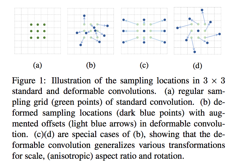
- deformable conv是从input到output的映射,映射可以是任意的transformation,且3x3x2的参数最多可以包含3x3种transformation
- sampling kernel对kernel内的每个点,也可以有不同的权重,也就是3x3个weight factor
- 还有啥跟形变相关的
- STN:
- attention机制
- spatial attention:STN,sSE
- channel attention:SENet
- 同时使用空间attention和通道attention机制:CBAM
papers
- [STN] STN: Spatial Transformer Networks,STN的变换是pre-defined的,是针对全局featuremap的变换
- [DCN 2017] Deformable Convolutional Networks ,DCN的变换是更随机的,是针对局部kernel分别进行的变化,基于卷积核添加location-specific shift
- [DCNv2 2018] Deformable ConvNets v2: More Deformable, Better Results,进一步消除irrelevant context,基于卷积核添加weighted-location-specific shift,提升performance
- [attention系列paper] [SENet &SKNet & CBAM & GC-Net][https://amberzzzz.github.io/2020/03/13/attention%E7%B3%BB%E5%88%97/]
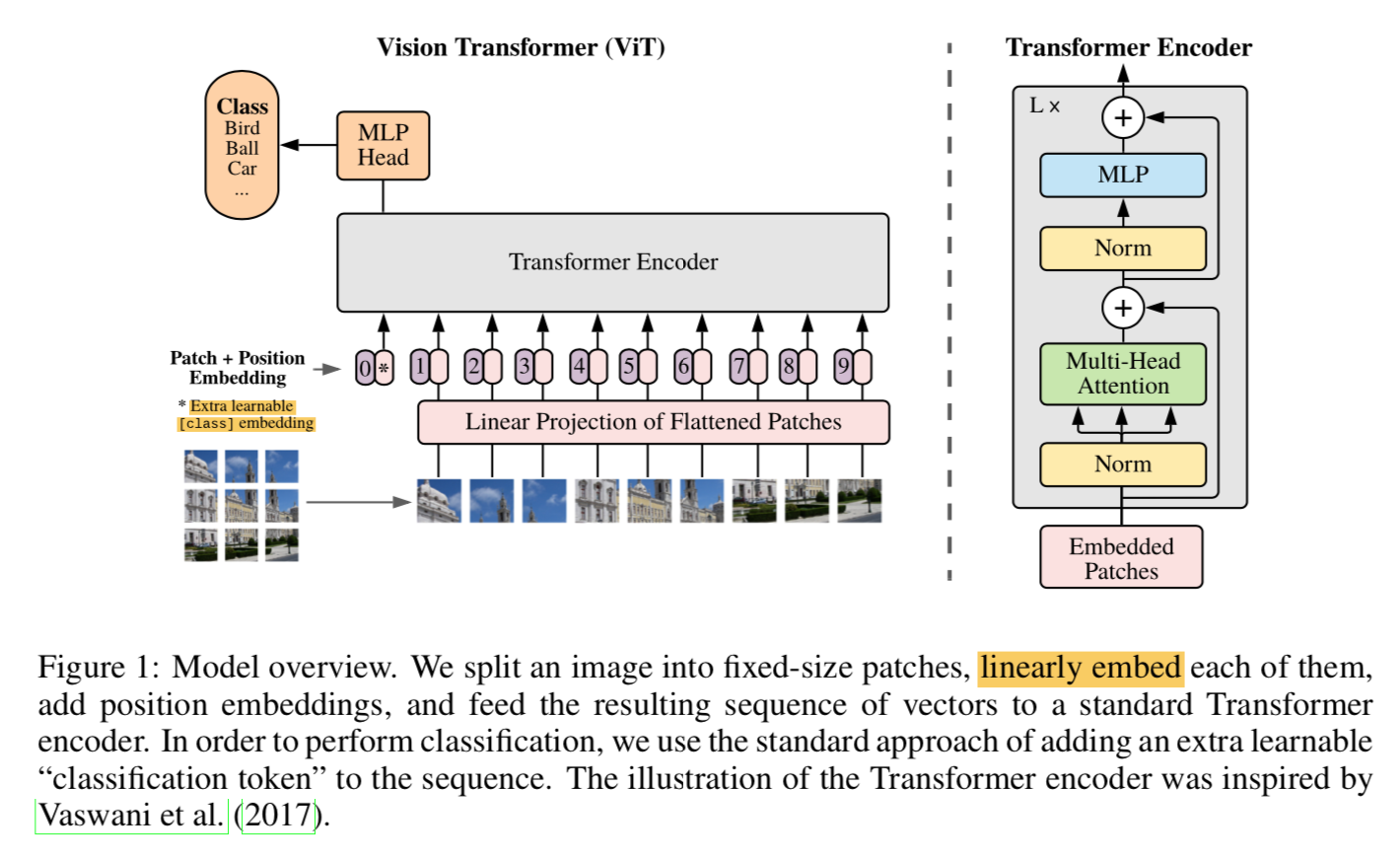
STN: Spatial Transformer Networks
动机
- 传统卷积:lack the ability of spacially invariant
- propose a new learnable module
- can be inserted into CNN
- spatially manipulate the data
- without any extra supervision
- models learn to be invariant to transformations
论点
- spatially invariant
- the ability of being invariant to large transformations of the input data
- max-pooling
- 在一定程度上spatially invariant
- 因为receptive fields are fixed and local and small
- 必须叠加到比较深层的时候才能实现,intermediate feature layers对large transformations不太行
- 是一种pre-defined mechanism,跟sample无关
- spatial transformation module
- conditioned on individual samples
- dynamic mechanism
- produce a transformation and perform it on the entire feature map
- task场景
- distorted digits分类:对输入做tranform能够simplify后面的分类任务
- co-localisation:
- spatial attention
- related work
- 生成器用来生成transformed images,从而判别器能够学习分类任务from transformation supervision
- 一些methods试图从网络结构、feature extractors的角度的获得invariant representations,while STN aims to achieve this by manipulating the data
- manipulating the data通常就是基于attention mechanism,crop涉及differentiable问题
- spatially invariant
方法
formulation
- localisation network:predict transform parameters
- grid generator:基于predicted params生成sampling grid
sampler:element-multiply
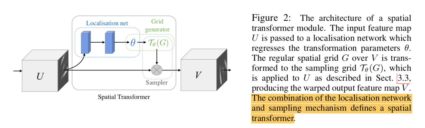
localisation network
- input feature map $U \in R^{hwc}$
- same transformation is applied to each channel
- generate parameters of transformation $\theta$:1-d vector
- fc / conv + final regression layer
parameterised sampling grid
sampling kernel
applied by pixel
general affine transformation:cropping,translation,rotation,scale,skew
ouput map上任意一点一定来自变换前的某一点,反之不一定,input map上某一点可能是bg,被crop掉了,所以pointwise transformation写成反过来的:

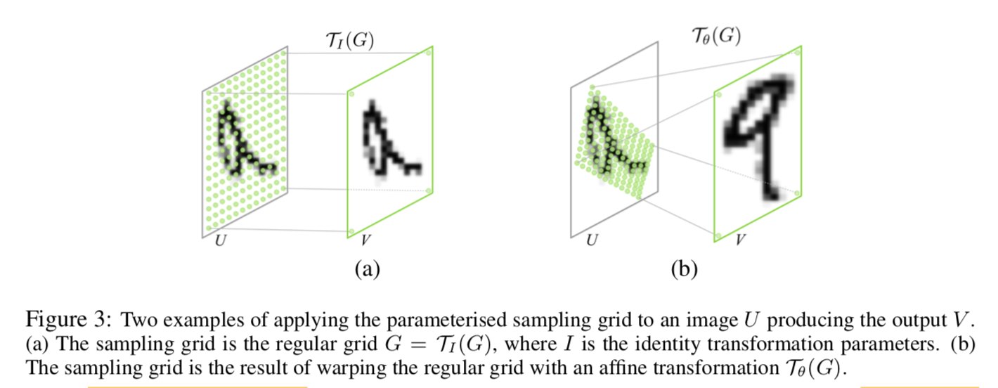
target points构成的点集就是sampling points on the input feature map
differentiable image sampling
通过上一步的矩阵transformation,得到input map上需要保留的source point set
对点集中每一点apply kernel
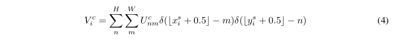
通用的插值表达式:
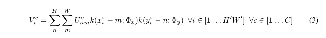
最近邻kernel是个pulse函数
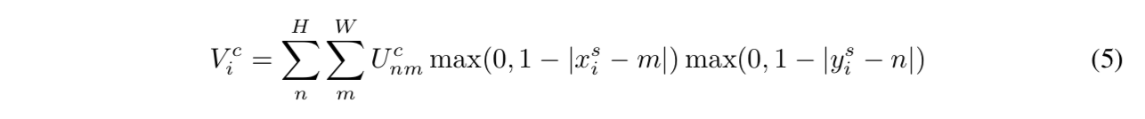
bilinear kernel是个distance>1的全mute掉,分段可导
STN:Spatial Transformer Networks
- 把spatial transformer嵌进CNN去:learn how to actively transform the features to help minimize the overall cost
- computationally fast
- 几种用法
- feed the output of the localization network $\theta$ to the rest of the network:因为transform参数explicitly encodes目标的位置姿态信息
- place multiple spatial transformers at increasing depth:串行能够让深层的transformer学习更抽象的变换
- place multiple spatial transformers in parallel:并行的变换使得每个变换针对不同的object
实验
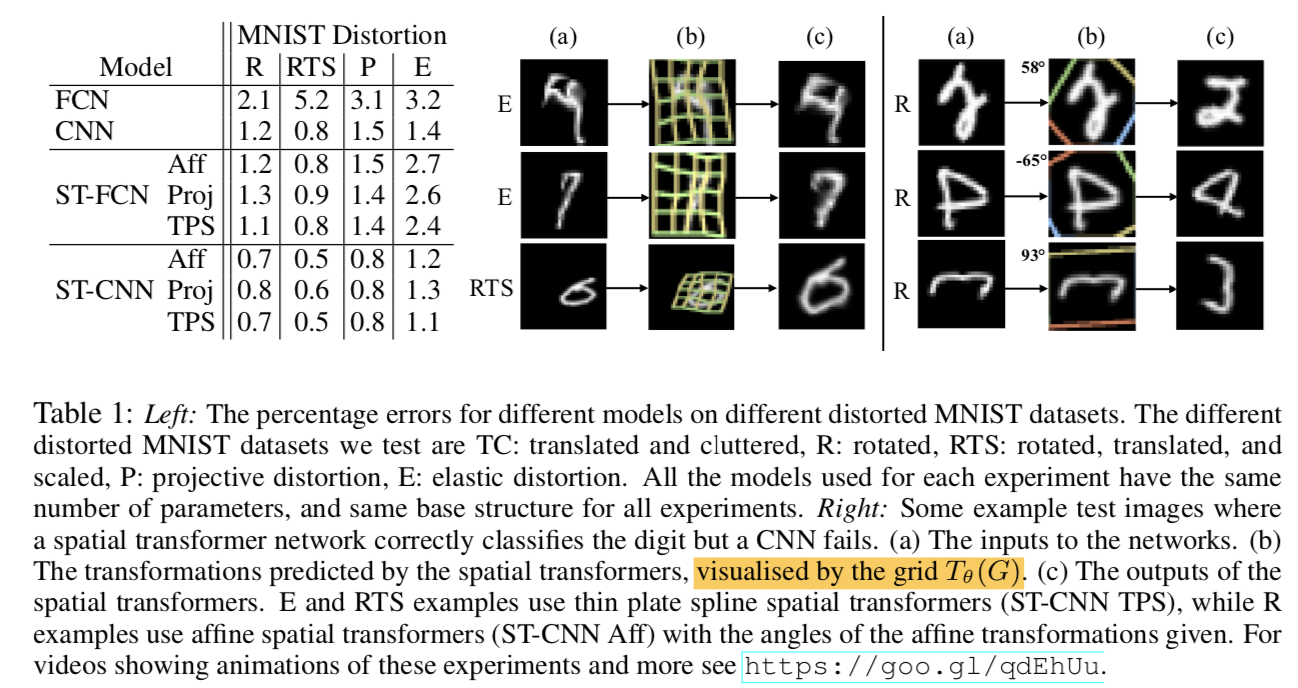
- R、RTS、P、E:distortion ahead
- aff、proj、TPS:transformer predefined
- aff:给定角度??
- TPS:薄板样条插值
Deformable Convolutional Networks
动机
- CNN:fixed geometric structures
- enhance the transformation modeling capability
- deformable convolution
- deformable RoI pooling
- without additional supervision
- share similiar spirit with STN
论点
to accommodate geometric variations
- data augmentation is limited to model large, unknown transformations
- fixed receptive fields is undesirable for high level CNN layers that encode the semantics
- 使用大量增广的数据,枚举不全,而且收敛慢,所需网络参数量大
- 对于提取语义特征的高层网络来讲,固定的感受野对不同目标不友好
introduce two new modules
- deformable convolution
- learning offsets for each kernel via additional convolutional layers
deformable RoI pooling
- learning offset for each bin partition of the previous RoI pooling
- deformable convolution
方法
overview
- operate on the 2D spatial domain
- remains the same across the channel dimension
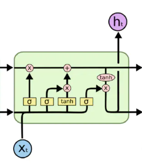
deformable convolution
- 正常的卷积:
- $y(p_0) = \sum w(p_n)*x(p_0 + p_n)$
- $p_n \in R\{(-1,-1),(-1,0),…, (0,0), (1,1)\}$
- deformable conv:with offsets $\Delta p_n$
- $y(p_0) = \sum w(p_n)*x(p_0 + p_n + \Delta p_n)$
- offset value is typically fractional
- bilinear interpolation:
- $x(p) = \sum_q G(q,p)x(q)$
- 其中$G(q,p)$是条件:$G(q,p)=max(0, 1-|q_x-p_x|)*max(0, 1-|q_y-p_y|)$
- 只计算和offset点距离小于1个单位的邻近点
- 实现
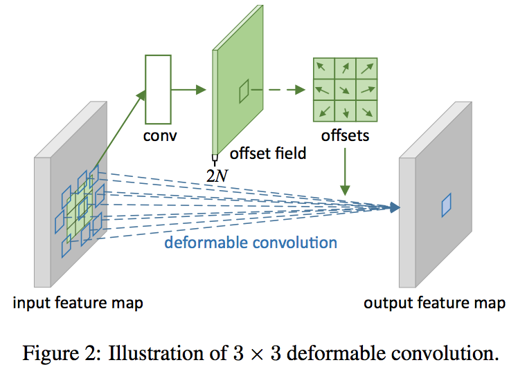
- offsets conv和特征提取conv是一样的kernel:same spatial resolution and dilation(N个position)
- the channel dimension 2N:因为是x和y两个方向的offset
- 正常的卷积:
deformable RoI pooling
RoI pooling converts an input feature map of arbitrary size into fixed size features
常规的RoI pooling
- divides ROI into k*k bins and for each bin:$y(i,j) = \sum_{p \in bin(i,j)} x(p_0+p)/n_{ij}$
- 对feature map上划分到每个bin里面所有的点
deformable RoI pooling:with offsets $\Delta p_{ij}$
- $y(i,j) = \sum_{p \in bin(i,j)} x(p_0+p+\Delta p_{ij})/n_{ij}$
- scaled normalized offsets:$\Delta p_{ij} = \gamma \Delta p_{ij} (w,h) $
- normalized offset value is fractional
- bilinear interpolation on the pooled map as above
实现
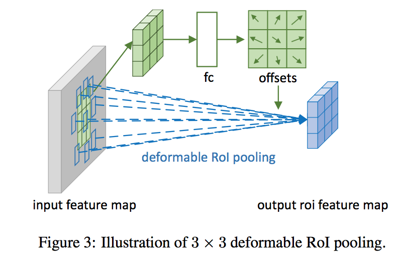
- fc layer:k*k*2个element(sigmoid?)
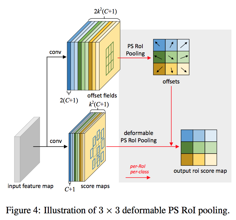
position sensitive RoI Pooling
- fully convolutional
- input feature map先通过卷积扩展成k*k*(C+1)通道
对每个C+1(包含kk个feature map),conv出全图的offset(2\k*k个)
deformable convNets
- initialized with zero weights
- learning rates are set to $\beta$ times of the learning rate for the existing layers
- $\beta=1.0$ for conv
- $\beta=0.01$ for fc
- feature extraction
- back:ResNet-101 & Aligned-Inception-ResNet
- withoutTop:A randomly initialized 1x1 conv is added at last to reduce the channel dimension to 1024
- last block
- stride is changed from 2 to 1
- the dilation of all the convolution filters with kernel size>1 is changed from 1 to 2
- Optionally last block
- use deformable conv in res5a,b,c
- segmentation and detection
- deeplab predicts 1x1 score maps
- Category-Aware RPN run region proposal with specific class
- modified faster R-CNN:add ROI pooling at last conv
- optional faster R-CNN:use deformable ROI pooling
- R-FCN:state-of-the-art detector
- optional R-FCN:use deformable ROI pooling
实验
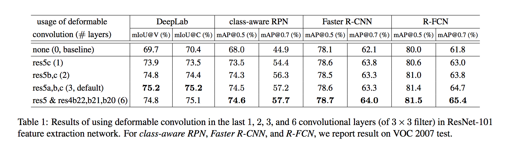
Accuracy steadily improves when more deformable convolution layers are used:使用越多层deform conv越好,经验取了3
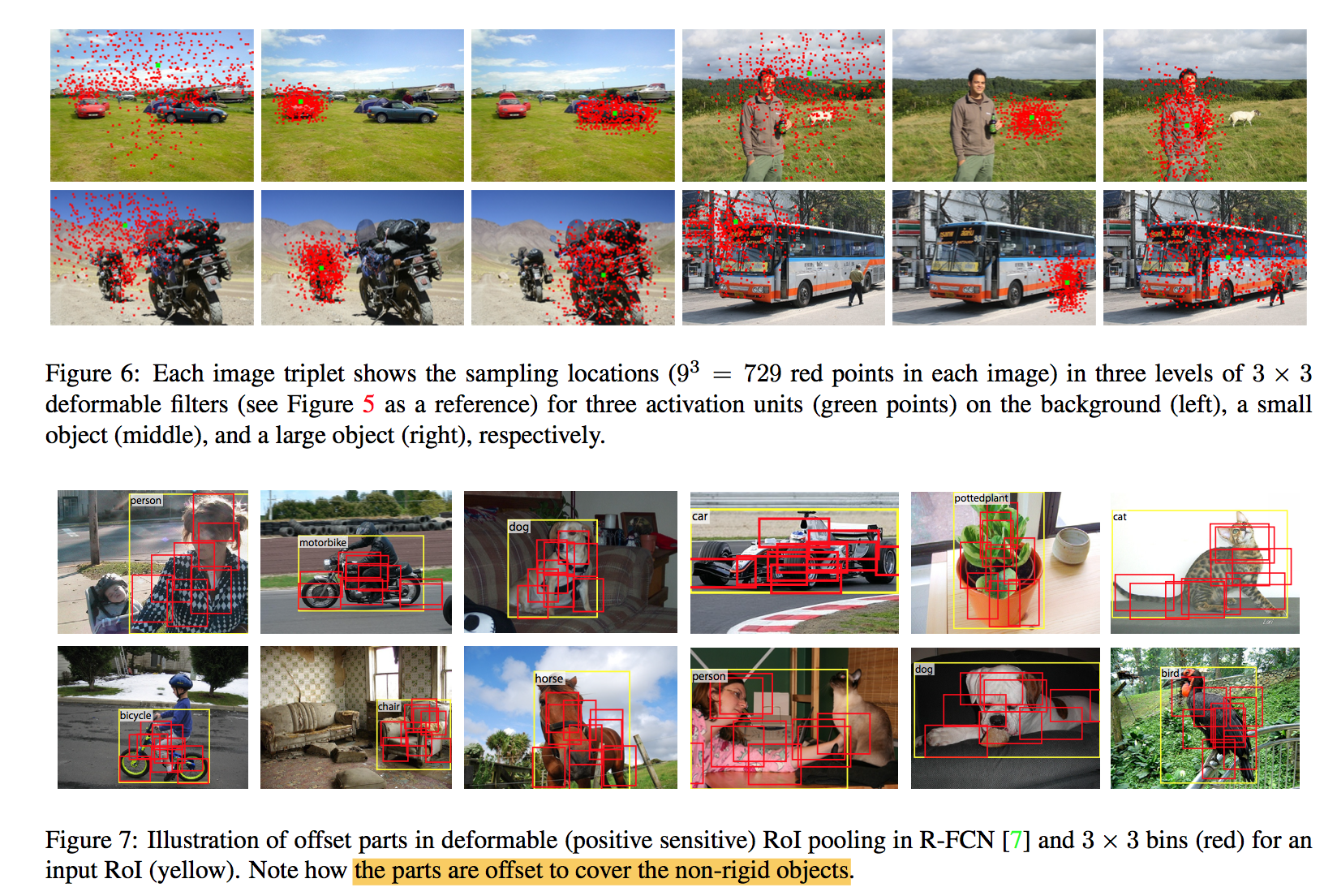
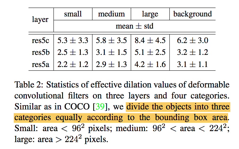
the learned offsets are highly adaptive to the image content:大目标的间距大,因为reception field大,consistent in different layers
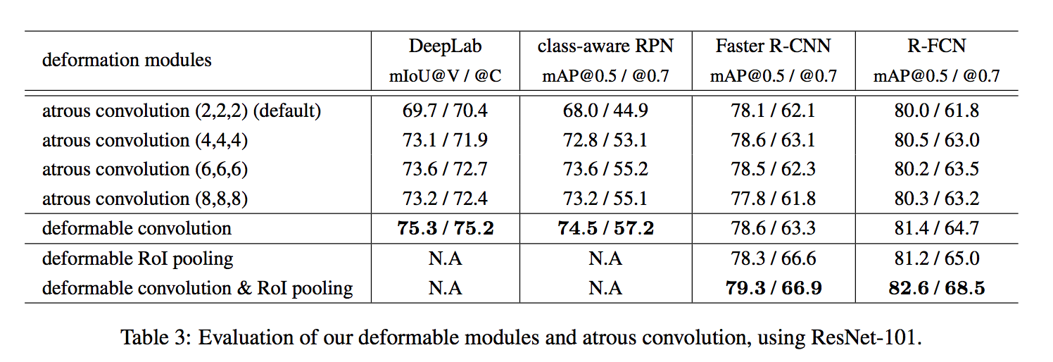
atrous convolution also improves:default networks have too small receptive fields,但是dilation需要手调到最优
using deformable RoI pooling alone already produces noticeable performance gains, using both obtains significant accuracy improvements
Deformable ConvNets v2: More Deformable, Better Results
动机
- DCN能够adapt一定的geometric variations,但是仍存在extend beyond image content的问题
- to focus on pertinent image regions
- increased modeling power
- more deformable layers
- updated DCNv2 modules
- stronger training
- propose feature mimicking scheme
- increased modeling power
- verified on
- incorporated into Faster-RCNN & Mask RCNN
- COCO for det & set
- still lightweight and easy to incorporate
论点
- DCNv1
- deformable conv:在standard conv的基础上generate location-specific offsets which are learned from the preceding feature maps
- deformable pooling:offsets are learned for the bin positions in RoIpooling
- 通过可视化散点图发现有部分散点落在目标外围
- propose DCNv2
- equip more convolutional layers with offset
- modified module
- each sample not only undergoes a learned offset
- but also a learned feature amplitude
- effective trainin
- use RCNN as the teacher network since RCNN learns features unaffected by irrelevant info outside the ROI
- feature mimicking loss
- DCNv1
方法
stacking more deformable conv layers
- replace more regular conv layers by their deformable counterparts:
- resnet50的stage3、4、5的3x3conv都替换成deformable conv:13个conv layer
- DCNv1是把stage5的3个resblock的3x3 conv替换成deformable conv:3个deconv layer
- 因为DCNv1里面在PASCAL上面实验发现再多的deconv精度就饱和了,但是DCNv2是在harder dataset COCO上面的best-acc-efficiency-tradeoff
- replace more regular conv layers by their deformable counterparts:
modulated deformable conv
- modulate the input feature amplitudes from different spacial locations/bins
- set the learnable offset & scalar for the k-th location:$\Delta p_k$和$\Delta m_k$
- set the conv kernel dilation:$p_k$,resnet里面都是1
- the value for location p is:$y(p) = \sum_{k=1}^K w_k x(p+p_k+\Delta p_k)\Delta m_k$,bilinear interpolation
- 目的是抑制无关信号
- learnable offset & scalar obtained via a separate conv layer over the same input feature map x
- 输出有3K个channel:2K for xy-offset,K for scalar
- offset的conv后面没激活函数,因为范围无限
- scalar的conv后面有个sigmoid,将range控制在[0,1]
- 两个conv全0初始化
- 两个conv layer的learning rate比existing layers小一个数量级
- modulate the input feature amplitudes from different spacial locations/bins
modulated deformable RoIpooling
- given an input ROI
- split into K(7x7) spatial bins
- average pooling over the sampling points for each bin计算bin的value
- the bin value is:$y(k) = \sum_{j=1}^{n_k} x(p_{kj}+\Delta p_k)\Delta m_k /n_k$,bilinear interpolation
- a sibling branch
- 2个1024d-fc:gaussian initialization with 0.01 std dev
- 1个3Kd-fc:全0初始化
- last K channels + sigmoid
- learning rate跟existing layers保持一致
RCNN feature mimicking
- 发现无论是conv还是deconv,error-bound都很大
- 尽管从设计思路上,DCNv2是带有mute irrelevant的能力的,但是事实上并没做到
- 说明such representation cannot be learned well through standard FasterRCNN training procedure:
- 说白了就是supervision力度不够
- 需要additional guidance
feature mimic loss
enforced only on positive ROIs:因为背景类往往需要更长距离/更大范围的context信息
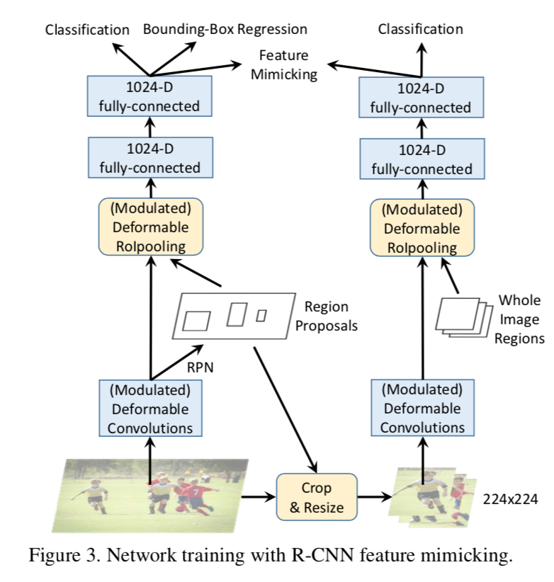
architecture
- add an additional RCNN branch
- RCNN input cropped images,generate 14x14 featuremaps,经过两个fc变成1024-d
- 和FasterRCNN里对应的counterpart,计算cosine similarity
这个太扯了不展开了