[LV-ViT 2021] Token Labeling: Training an 85.4% Top-1 Accuracy Vision Transformer with 56M Parameters on ImageNet,新加坡国立&字节,主体结构还是ViT,deeper+narrower+multi-layer-cnn-patch-projection+auxiliary label&loss
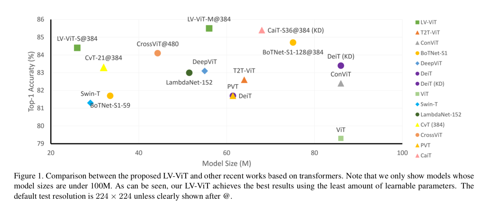
同等参数量下,能够达到与CNN相当的分类精度
- 26M——84.4% ImageNet top1 acc
- 56M——85.4% ImageNet top1 acc
- 150M——86.2% ImageNet top1 acc
ImageNet & ImageNet-1k:The ImageNet dataset consists of more than 14M images, divided into approximately 22k different labels/classes. However the ImageNet challenge is conducted on just 1k high-level categories (probably because 22k is just too much)
Token Labeling: Training an 85.4% Top-1 Accuracy Vision Transformer with 56M Parameters on ImageNet
动机
- develop a bag of training techniques on vision transformers
- slightly tune the structure
- introduce token labeling——a new training objective
- ImageNet classificaiton task
论点
- former ViTs
- 主要问题就是需要大数据集pretrain,不然精度上不去
- 然后模型也比较大,need huge computation resources
- DeiT和T2T-ViT探索了data augmentation/引入additional token,能够在有限的数据集上拉精度
- our work
- rely on purely ImageNet-1k data
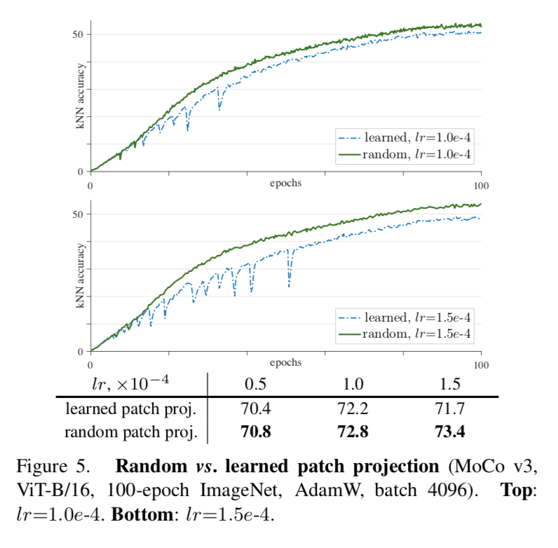
- rethink the way of performing patch embedding
- introduce inductive bias
- we add a token labeling objective loss beside cls token predition
- provide practical advice on adjusting vision transformer structures
- former ViTs
方法
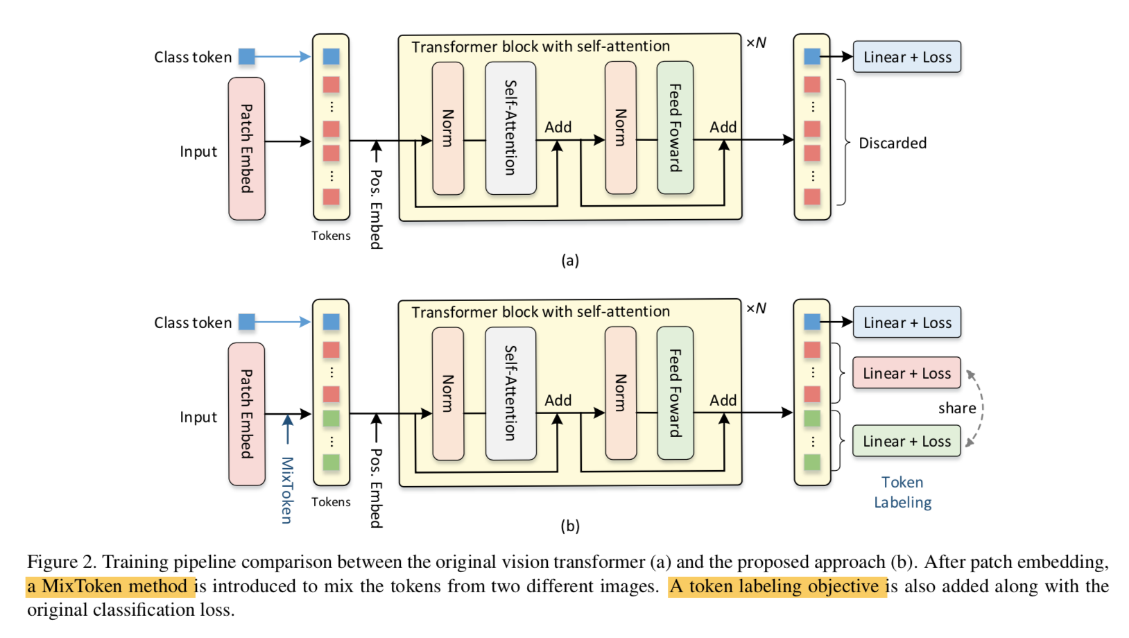
overview & comparison
- 主体结构不变,就是增加了两项
- a MixToken method
a token labeling objective
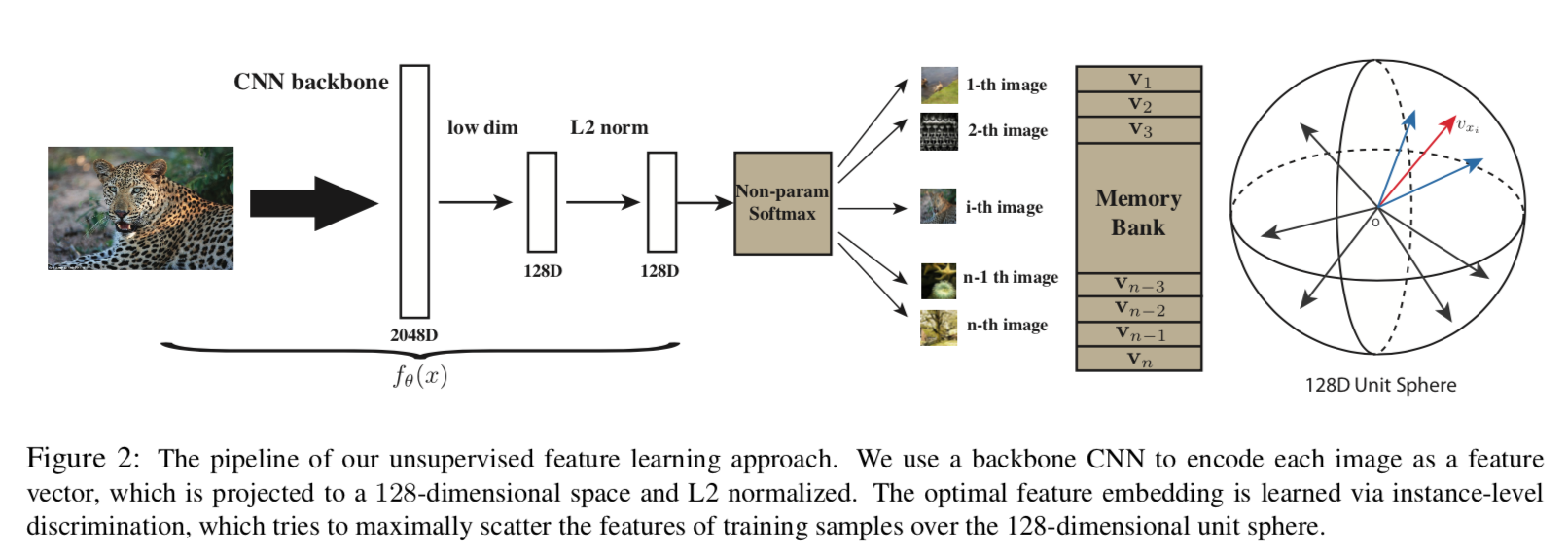
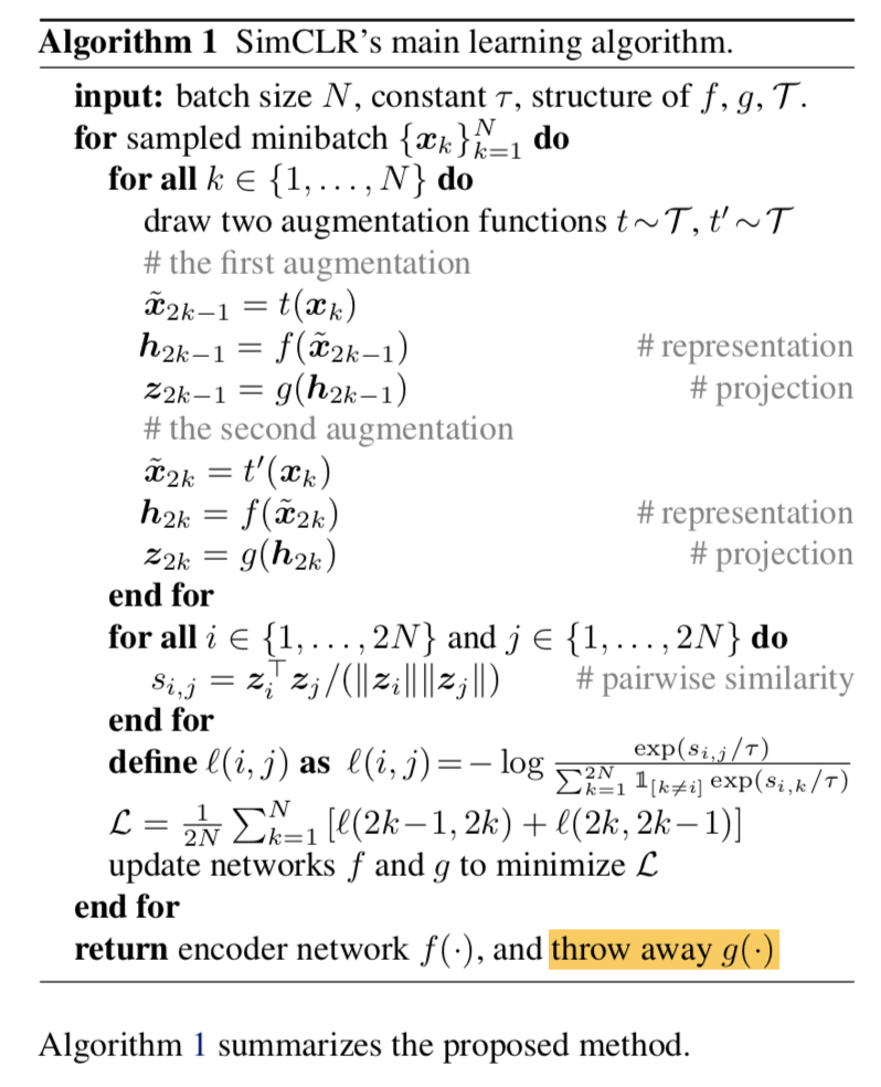
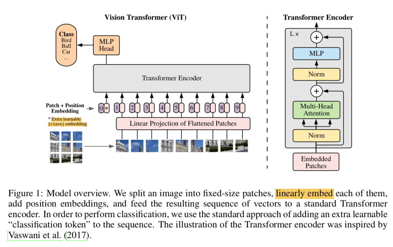
review the vision transformer
- patch embedding
- 将固定尺寸的图片转换成patch sequence,例如224x224的图片,patch size=16,那就是14x14个small patches
- 将每个patch(16x16x3=768-dim) linear project成一个token(embedding-dim)
- concat a class token,构成全部的input tokens
- position encoding
- added to input tokens
- fixed sinusoidal / learnable
- multi-head self-attention
- 用来建立long-range dependency
- multi-heads:所有attention heads的输出在channel-dim上concat,然后linear project回单个head的channel-dim
- feed-forward layers
- fc1-activation-fc2
- score predition layer
- 只用了cls token对应的输出embedding,其他的discard
- patch embedding
training techniques
network depth
- add more transformer blocks
- 同时decrease the hidden dim of FFN
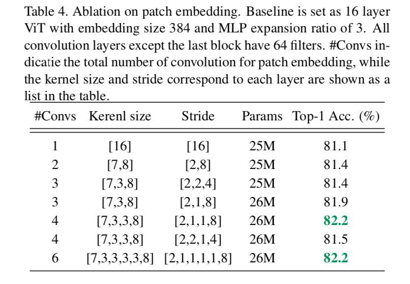
explicit inductive bias
- CNN逐步扩大感受野,擅长提取局部特征,具有天然的平移不变性等
- transformer被发现failed to capture the low-level and local structures
- we use convolutions with a smaller stride to provide an overlapped information for each nearby tokens
- 在patch embedding的时候不是independent crop,而是有overlap
- 然后用多层conv,逐步扩大感受野,smaller kernel size同时降低了计算量
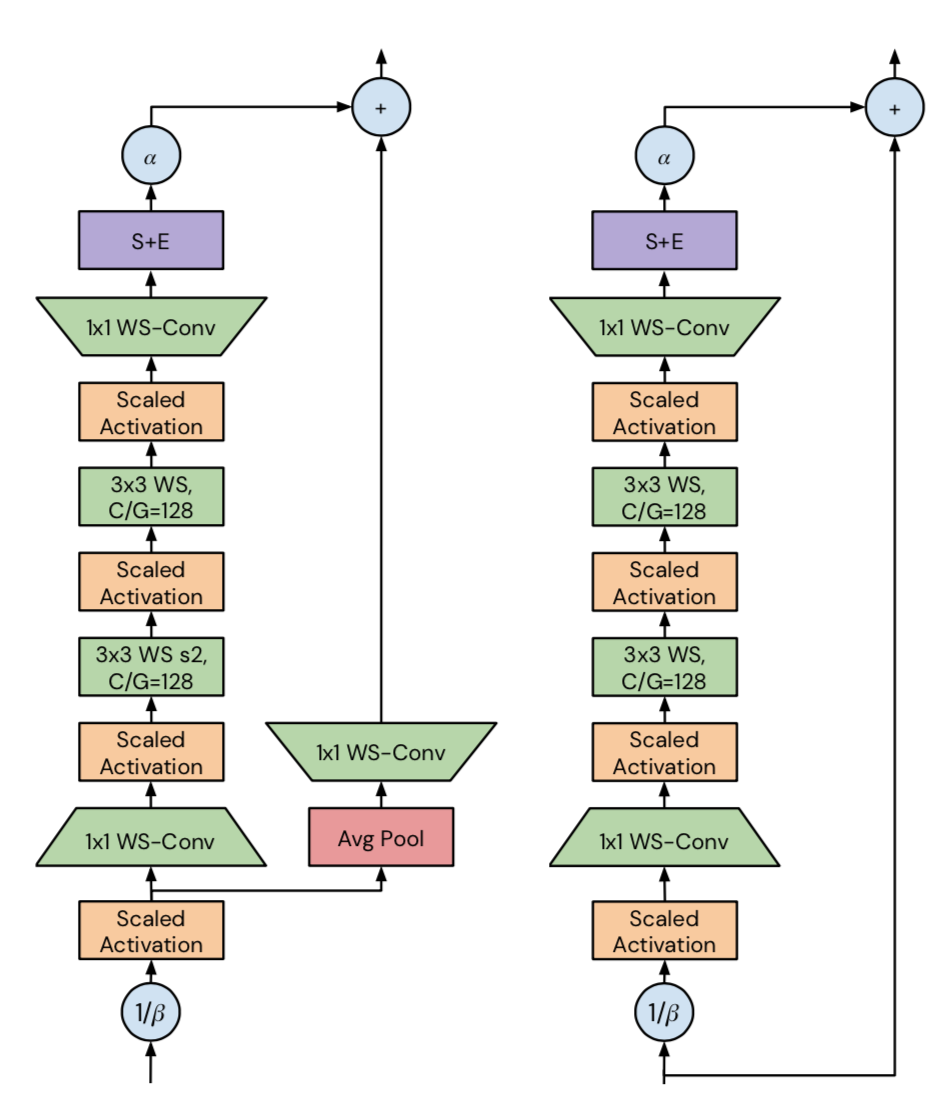
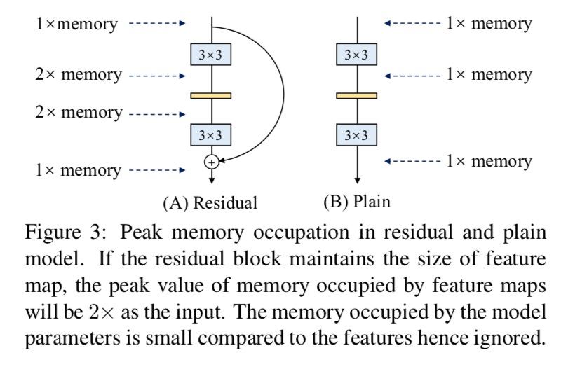
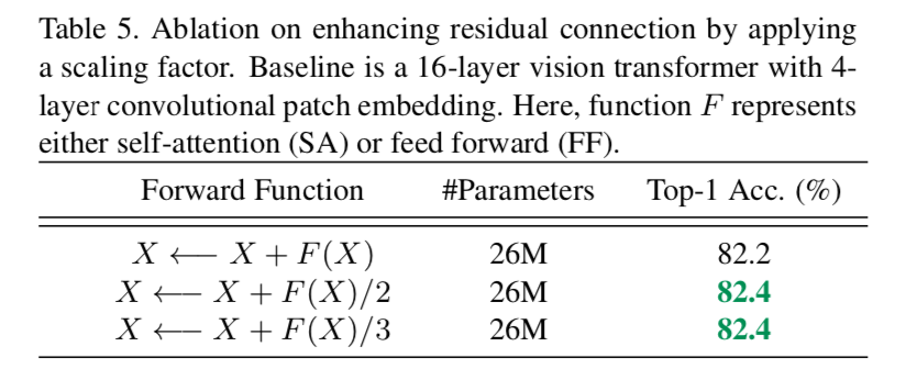
rethinking residual connection
给残差分支add a smaller ratio $\alpha$
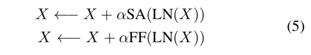
enhance the residual connection since less information will go to the residual branch
improve the generalization ability
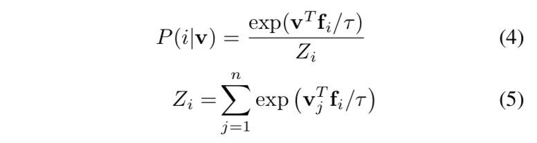
re-labeling
- label is not always accurate after cropping
situations are worse on smaller images
re-assign each image with a K-dim score map,在1k类数据集上K=1000
- cheap operation compared to teacher-student
- 这个label是针对whole image的label,是通过另一个预训练模型获取
token-labeling
- based on the dense score map provided by re-labeling,we can assign each patch an individual label
- auxiliary token labeling loss
- 每个token都对应了一个K-dim score map
- 可以计算一个ce
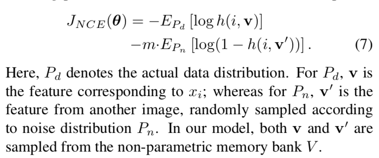
- given
- outputs of the transformer $[X^{cls}, X^1, …, X^N]$
- K-dim score map $[y^1, y^2, …, y^N]$
- whole image label $y^{cls}$
- loss
- auxiliary token labeling loss:$L_{aux} = \frac{1}{N} \sum_1^N CE(X^i, y^i)$
- cls loss:$L_{cls} = CE(X^{cls}, y^{cls})$
- total loss:$L_{total} = L_{cls}+\beta L_{aux}$,$\beta=0.5$
MixToken
- 从Mixup&CutMix启发来的
- 为了确保each token have clear content,我们基于token embedding进行mixup
- given
- token sequence $T_1=[t^1_1, t^2_1, …, t^N_1]$ & $T_2=[t^1_2, t^2_2, …, t^N_2]$
- token labels $y_1=[y^1_1, y^2_1, …, y^N_1]$ & $Y_2=[y^1_2, y^2_2, …, y^N_2]$
- binary mask M
- MixToken
- mixed token sequence:$\hat T = T_1 \odot M + T_2 \odot (1-M)$
- mixed labels:$\hat Y = Y_1 \odot M + Y_2 \odot (1-M)$
- mixed cls label:$\hat {Y^{cls}} = \overline M y_1^{cls} + (1-\overline M) y_2^{cls}$,$\overline M$ is the average of $M$
实验
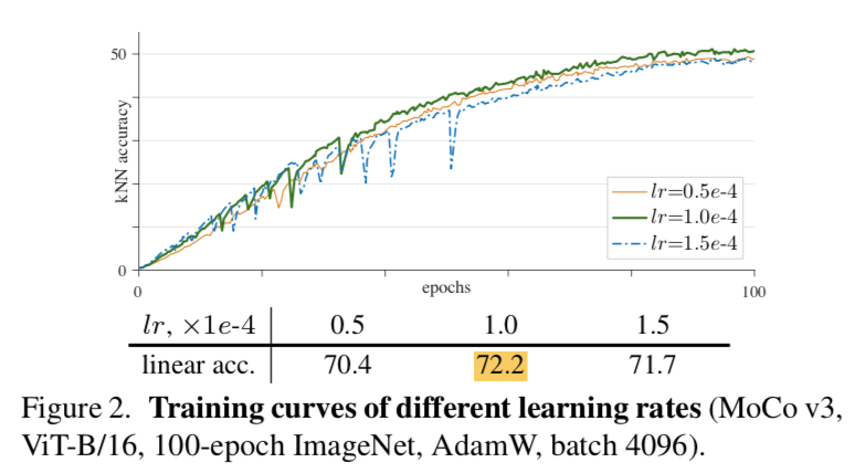
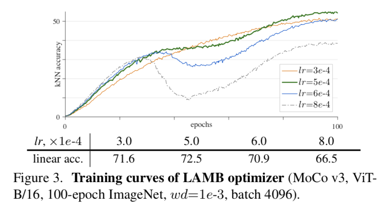
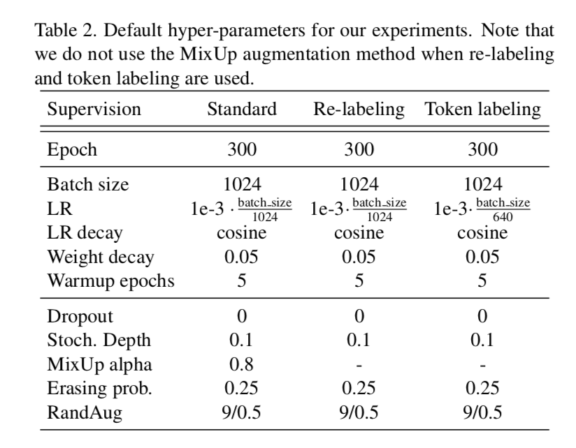
training details
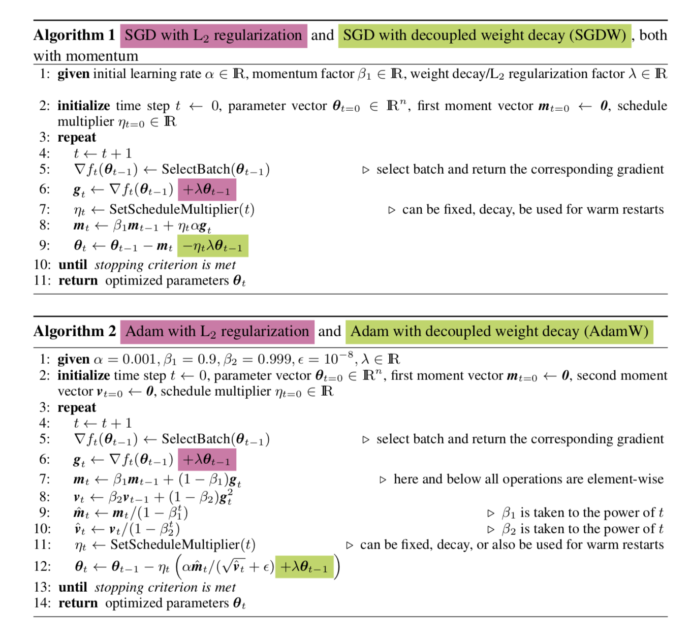
- AdamW
- linear lr scaling:larger when use token labeling
- weight decay
dropout:hurts small models,use Stochastic Depth instead
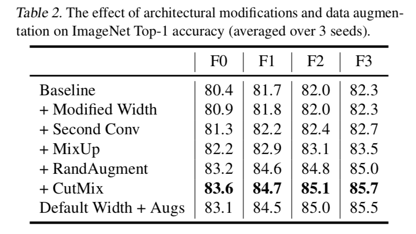
Training Technique Analysis
more convs in patch embedding
enhanced residual
smaller scaling factor
- the weight get larger gradients in residual branch
- more information can be preserved in main branch
- better performance
- faster convergence
re-labeling
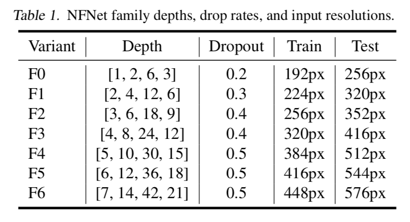
- use NFNet-F6 to re-label the ImageNet dataset and obtain the 1000-dimensional score map for each image
- NFNet-F6 is trained from scratch
- given input 576x576,获得的score map是18x18x1000(s32)
- store the top5 probs for each position to save storage
MixToken
- 比baseline的CutMix method要好
同时看到token labeling比relabeling要好
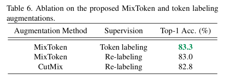
token labeling
- relabeling是在whole image上
- token labeling是进一步地,在token level添加label和loss
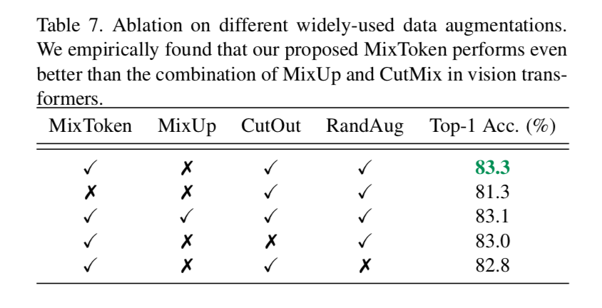
augmentation techniques
发现MixUp会hurt
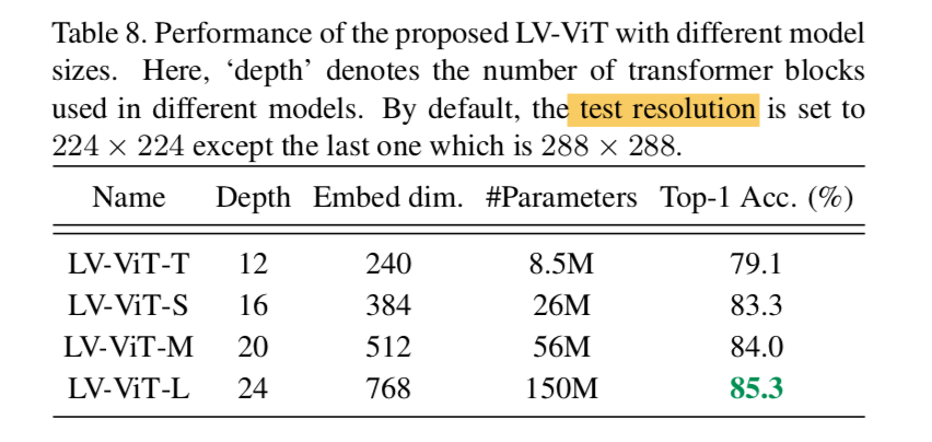
Model Scaling
越大越好