reference：https://zhuanlan.zhihu.com/p/32903856

引用量：4193

R-FCN: Object Detection via Region-based Fully Convolutional Networks

1. 动机

   • region-based：
     • 先框定region of interest的检测算法
     • previous methods：Fast/Faster R-CNN，apply costly per-region subnetwork hundreds of times
   • fully convolutional
     • 旨在解决Faster R-CNN第二阶段计算不共享，效率低的问题
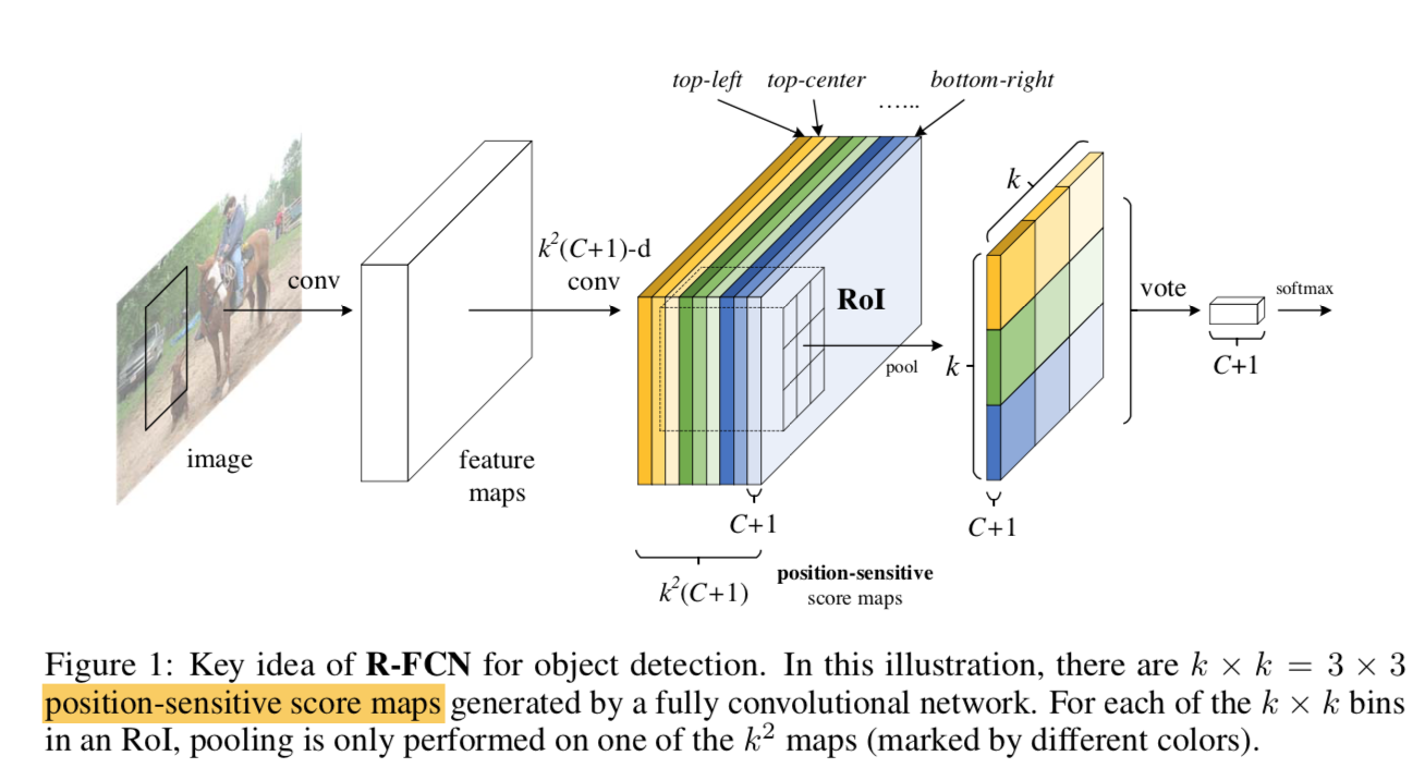
   • we propose position-sensitive score maps
     • translation-invariance in image classification
     • translation-variance in object detection
   • verified on PASCAL VOC

2. 论点

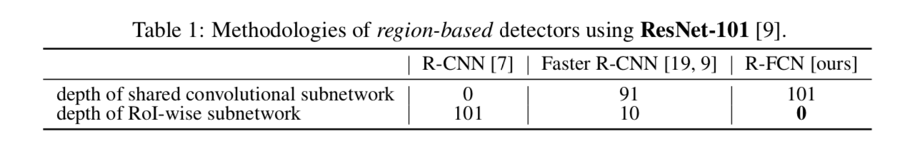
   • 主流的两阶段检测架构

     • two subnetworks

       • a shared fully convolutional：这一部分提取通用特征，作用于全图
       • an RoI-wise subnetwork：这一部分不能共享计算，作用于proposals，因为是要针对每个位置的ROI进行分类和回归

       • 也就是说，第一部分是位置不敏感的，第二部分是位置敏感的

         

     • 网络越深越translation invariant，目标怎么扭曲、平移最终的分类结果都不变，多层pooling后的小feature map上也感知不到小位移，平移可变性（translation variance），对定位任务不友好

     • 所以resnet-back-detector我们是把ROI Pooling放在stage4后面，跟一个RoI-wise的stage5

       • improves accuracy
       • lower speed due to RoI-wise

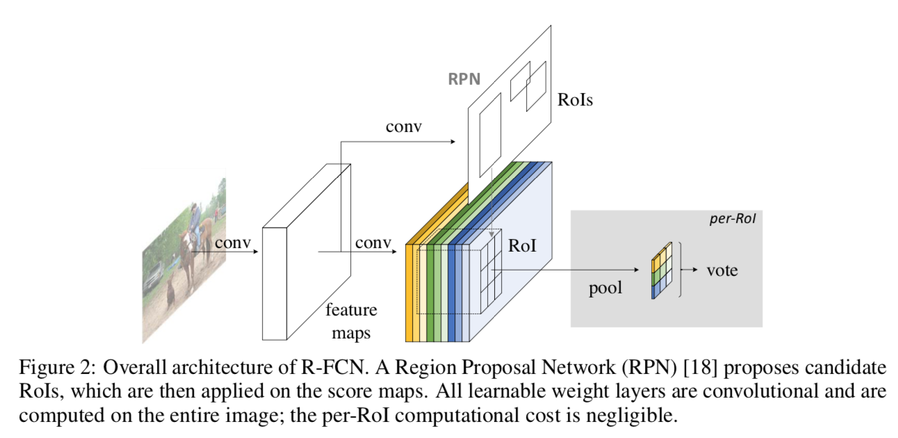
   • R-FCN

     • 要解决的根本问题是RoI-wise部分不共享，速度慢：300个proposal要计算300次
     • 单纯地将网络提前放到shared back里面不行，会造成translation invariant，位置精度会下降

     • 必须通过其他方法加强网络的平移可变性，所以提出了position-sensitive score map

       • 将全图划分为kxk个区域
       • position-sensitive score map：生成kxkx(C+1)个特征图
       • 每个位置对应C+1个特征图
       • 做RoIPooling的时候，每个bin来自每个position对应的C+1个map（这咋想的，space dim到channel dim再到space dim？）

       

3. 方法

   • overview

     

     • two-stage
       • region proposal：RPN
       • region classification：the R-FCN
     • R-FCN
       • 全卷积
       • 输出conv层有kxkx(C+1)个channel
         • kxk对应grid positions
         • C+1对应C个前景+background
       • 最后是position-sensitive RoI pooling layer
         • aggregates from last conv and RPN？
         • generate scores for each RoI
         • each bin aggregates responses from对应的position的channel score maps，而不是全部通道
         • force模型在通道上形成对不同位置的敏感能力

   • R-FCN architecture

     • back：ResNet-101，pre-trained on ImageNet，block5 输出是2048-d
     • 然后接了random initialized 1x1 conv，降维
     • cls brach
       • 接$k^2(C+1)$的conv生成score maps
       • 然后是Position-sensitive RoI pooling
         • 将每个ROI均匀切分成kxk个bins
         • 每个bin在对应的Position-sensitive score maps中找到唯一的通道，进行average pooling
         • 最终得到kxk的pooling map，C+1个通道
         • 将pooling map performs average pooling，得到C+1的vector，然后softmax
     • box branch
       • 接$4k^2$的conv生成score maps
       • Position-sensitive RoI pooling
         • 得到kxk的pooling map，4个通道
         • average pooling，得到4d vector，作为回归值$(t_x,t_y,t_w,t_h)$
     • there is no learnable layer after the ROI layer，enable nearly cost-free region-wise computation

   • Training

     • R-FCN positives / negatives：和gt box的IoU>0.5的proposasl
     • adopt OHEM
     • sort all ROI loss and select the highest 128
     • 其他settings基本和Faster-RCNN一致
   • Atrous and stride
     • 特别地，对resnet的block5进行了改变
     • stride2改成stride1
     • 所有的conv改成空洞卷积
     • RPN是接在block4的输出上，所以不受空洞卷积的影响，只影响R-FCN head

papers

• [MPL 2021] Meta Pseudo Labels

• [UDA 2009] Unsupervised Data Augmentation for Consistency Training

• [Entropy Minimization 2004] Semi-supervised Learning by Entropy Minimization

Meta Pseudo Labels

1. 动机

   • semi-supervised learning
     • Pseudo Labels：fixed teacher
     • Meta Pseudo Labels：constantly adapted teacher by the feedback of the student
   • SOTA on ImageNet：top-1 acc 90.2%

2. 论点

   • Pseudo Labels methods

     • teacher generates pseudo labels on unlabeled images
     • pseudo labeled images are then combined with labeled images to train the student
     • confirmation bias problem：student的精度取决于伪标签的质量

   • we propose Meta Pseudo Labels

     • teacher observes how its pseudo labels affect the student
     • then correct the bias
     • the feedback signal is the performance of the student on the labeled dataset
     • 总的来说，teacher和student是train in parallel的
       • student learns from pseudo labels from the teacher
       • teacher learns from reward signal from how well student perform on labeled set
     • dataset
       • ImageNet as labeled set
       • JFT-300M as unlabeled set
     • model
       • teacher：EfficientNet-L2
       • student：EfficientNet-L2

   • main difference

     • Pseudo Labels方法中，teacher在单向的影响student

     • Meta Pseudo Labels方法中，teacher和student是交互作用的

       

3. 方法

   • notations

     • models
       • teacher model T & $\theta_T$
       • student model S & $\theta_S$
     • data
       • labeled set $(x_l, y_l)$
       • unlabeled set $(x_u)$
     • predictions
       • soft predictions by teacher $T(x_u, \theta_T)$
       • student $S(x_u, \theta_S)$ & $S(x_l, \theta_S)$
     • loss
       • $CE(q,p)$，其中$q$是one-hot label，e.g. $CE(y_l, S(x_l, \theta_S))$

   • Pseudo Labels

     • given a fixed teacher $\theta_T$

     • train the student model to minimize the cross-entropy loss on unlabeled data

       $$\theta_S^{PL} = argmin_{\theta_S}CE(T(x_u,\theta_T), S(x_u, \theta_S))$$

     • $\theta_S^{PL}$ also achieve a low loss on labeled data

     • $\theta_S^{PL}$ explicitly depends on $\theta_T$：$\theta_S^{PL}(\theta_T)$
     • student loss on labeled data is also a function of $\theta_T$：$L_l(\theta_S^{PL}(\theta_T))$

   • Meta Pseudo Labels

     • intuition：minimize $L_l$ with respect to $\theta_T$

     • 但是实际上dependency of $\theta_S^{PL}(\theta_T)$ on $\theta_T$ 非常复杂

     • 因为我们用了teacher prediction的hard labels去训练student

     • an alternating optimization procedure

       

     • teacher’s auxiliary losses

       • augment the teacher’s training with a supervised learning objective and a semi-supervise learning objective
       • supervised objective
         • train on labeled data
         • CE
       • semi-supervised objective
         • train on unlabeled data
         • UDA(Unsupervised Data Augmentation)：将样本进行简单增强，通过衡量一致性损失，模型的泛化效果得到提升
         • consistency training loss：KL散度

     • finetuning student

       • 在meta pseudo labels训练过程中，student only learns from the unlabeled data
       • 所以在训练过程结束后，可以finetune it on labeled data to improve accuracy

     • overall algorithm

       

         * 这里面有一处下标写错了，就是teacher的UDA gradient，是在unlabeled data上面算的，那两个$x_l$得改成$x_u$
         * UDA loss论文里使用两个predicted logits的散度，这里是CE
       

Unsupervised Data Augmentation for Consistency Training

1. 动机

   • data augmentation in previous works
     • 能在一定程度上缓解需要大量标注数据的问题
     • 多用在supervised model上
     • achieved limited gains
   • we propose UDA
     • apply data augmentation in semi-supervised learning setting
     • use harder and more realistic noise to generate the augmented samples
     • encourage the prediction to be consistent between unlabeled & augmented unlabeled sample
     • 在越小的数据集上提升越大
   • verified on
     • six language tasks
     • three vision tasks
       • ImageNet-10%：：top1/top5 68.7/88.5%
       • ImageNet-extra unlabeled：top1/top5 79.0/94.5%

2. 论点

   • semi-supervised learning
     • three categories
       • graph-based label propagation via graph convolution and graph embeddings
       • modeling prediction target as latent variables
       • consistency / smoothness enforcing
     • 最后这一类方法shown to work well，
       • enforce the model predictions on the two examples to be similar
       • 主要区别在于perturbation function的设计
   • we propose UDA
     • use state-of-the-art data augmentation methods
     • we show that better augmentation methods(AutoAugment) lead to greater improvements
     • minimizes the KL divergence
     • can be applied even the class distributions of labeled and unlabeled data mismatch
   • we propose TSA
     • a training technique
     • prevent overfitting when much more unlabeled data is avaiable than labeled data

3. 方法

   • formulation

     • given an input $x\in U$ and a small noise $\epsilon$

     • compute the output distribution $p_{\theta}(y|x)$ and $p_{\theta}(y|x,\epsilon)$

     • minimize the divergence between two predicted distributions $D(p_{\theta}(y|x)||p_{\theta}(y|x,\epsilon))$

       

     • add a CE loss on labeled data

       

     • UDA的优化目标

       • enforce the model to be insensitive to perturbation
       • thus smoother to the changes in the input space

     • $\lambda=1$ for most experiments

     • use different batchsize for labeled & unlabeled

   • Augmentation Strategies for Different Tasks

     • AutoAugment for Image Classification
       • 通过RL搜出来的一组optimal combination of aug operations
     • Back translation for Text Classification
     • TF-IDF based word replacing for Text Classification

   • Trade-off Between Diversity and Validity for Data Augmentation

     • 对原始sample做变换的时候，有一定概率导致gt label变化
     • AutoAugment已经是optmial trade-off了，所以不用管
     • text tasks需要调节temperature

   • Additional Training Techniques

     • TSA(Training Signal Annealing)

       • situation：unlabeled data远比labeled data多的情况，我们需要large enough model去充分利用大数据，但又容易对小trainset过拟合

       • for each training step

         • set a threshold $\frac{1}{K}\leq \eta_t\leq 1$，K is the number of categories
         • 如果样本在gt cls上的预测概率大于这个threshold，就把这个样本的loss去掉

       • $\eta_t$ serves as a ceiling to prevent the model from over-training on examples that the model is already confident about

       • gradually release the training signals of the labeled examples，缓解overfitting

       • schedules of $\eta_t$

         • log-schedule：$\lambda_t = 1-exp(-\frac{t}{T}*5)$
         • linear-schedule：$\lambda_t = \frac{t}{T}$

         • exp-schedule：$\lambda_t = exp((\frac{t}{T}-1)*5)$

         • 如果模型非常容易过拟合，用exp-schedule，反过来（abundant labeled data/effective regularizations），用log-schedule

           

     • Sharpening Predictions

       • situation：the predicted distributions on unlabeled examples tend to be over-flat across categories，task比较困难，训练数据比较少时，在unlabeled data上每类的预测概率都差不多低，没有倾向性
       • 这时候KL divergence的监督信息就很弱
       • thus we need to sharpen the predicted distribution on unlabeled examples
       • Confidence-based masking：将current model not confident enough to predict的样本过滤掉，只保留最大预测概率大于0.6的样本计算consistency loss
       • Entropy minimization：add an entropy term to the overall objective
       • softmax temperature：在计算softmax时先对logits进行rescale，$Softmax(logits/\tau)$，a lower temperature corresponds to a sharper distribution
       • in practice发现Confidence-based masking和softmax temperature更适用于小labeled set，Entropy minimization适用于相对大一点的labeled set

     • Domain-relevance Data Filtering

       • 其实也是Confidence-based masking，先用labeled data训练一个base model，然后inference the out-of-domain dataset，挑出预测概率较大的样本

Semi-supervised Learning by Entropy Minimization

Generalized Focal Loss: Learning Qualified and Distributed Bounding Boxes for Dense Object Detection

1. 动机

   • one-stage detectors
     • dense prediction
     • three fundamental elements
       • class branch
       • box localization branch
       • an individual quality branch to estimate the quality of localization
   • current problems
     • the inconsistent usage of the quality estimation in train & test
     • the inflexible Dirac delta distribution：将box regression的value建模成真值附近的脉冲分布，用来描述边界不清晰/遮挡的case可能不准确
   • we design new representations for these three elements
     • merge quality estimation into class prediction：将objectness/centerness整合进cls prediction，直接用作NMS score
     • continout labels
     • propose GFL(Generalized Focal Loss) that generalizes Focal Loss from discrete form into continous version
   • test on COCO
     • ResNet-101-?-GFL: 45.0% AP
     • defeat ATSS

2. 论点

   • inconsistent usage of localization quality estimation and classification score

     • 训练的时候quality和cls branch是independent branch
     • box branch的supervision只作用在positive样本上：which is unreliable on predicting negatives
     • 测试阶段将quality和cls score乘起来有可能拉高负样本的分数，以至于在NMS阶段把低分正样本挤掉

   • inflexible representation of bounding boxes

     • most method建模成脉冲分布：只在IoU大于一定阈值的格子上有响应，别的格子都是0
     • some recent work建模成高斯分布
     • in fact the real distribution can be more arbitrary and flexible，连续且不严格镜像

   • thus we propose

     • merge the quality representation into the class branch：

       • class vector的每个元素代表了格子的localization quality(如IoU score)

       • 在inference阶段也是直接用作cls score

         

     • propose arbitrary/general distribution

       • 有明确边界的目标的边的分布是比较sharp的

       • 没有明显边界的边分布就是flatten一点

         

     • Generalized Focal Loss (GFL)

       • joint class representation是continuous IoU label (0∼1)
       • imbalance问题仍然存在，但是standart Focal Loss仅支持[0,1] sample
       • 修改成continuous形式，同时specialized into Quality Focal Loss (QFL) and Distribution Focal Loss (DFL)
         • QFL for cls branch：focuses on a sparse set of hard examples
         • DFL for box branch： focus on learning the probabilities of values around the continuous target locations

3. 方法

   • Focal Loss (FL)

     

     • standard CE part：$-log(p_t)$
     • scaling factor：down-weights the easy examples，focus on hard examples

   • Quality Focal Loss (QFL)

     • soft one-hot label：正样本在对应类别上有个(0,1]的float score，负样本全0

     • float score定义为预测框和gt box的IoU score

     • we adopt multiple binary classification with sigmoid

     • modify FL

       • CE part 改成complete form：$-ylog(\hat y)-(1-y)log(1-\hat y)$
       • scaling part用vector distance替换减法：$|y-\hat y |^{\beta}$

       • $\beta$ controls the down-weighting rate smoothly & $\beta=2$ works best

         

   • Distribution Focal Loss (DFL)

     • use relative offsets from the location to the four sides of a bounding box as the regression targets

     • 回归问题formulation

       • 连续：$\hat y = \int_{y_0}^{y_n}P(x)xdx$
       • 离散化：$\hat y = \sum_{i=0}^n P(y_i)y_i$
       • P(x) can be easily implemented through a softmax layer containing n+1 units：

     • DFL

       • force predictions to focus values near label $y$：explicitly enlarge the probabilities of $y_i$和$y_{i+1}$，given $y_i \leq y \leq y_{i+1}$
       • $log(S_i)$ force the probabilities

       • gap balance the 上下限，使得$\hat y$的global mininum solution无限逼近真值$y$，如果真值接近的是$\hat y_{i+1}$，可以看到$log(S_i)$那项被downscale了

         

   • Generalized Focal Loss (GFL)

     

     • 以前的cls preditions在测试阶段要结合quality predictions作为NMS score，现在直接就是

     • 以前regression targets每个回归一个值，现在是n+1个值

     • overall

       

       • 第一项cls loss，就是QFL，dense on 所有格子，用正样本数去norm
       • 第二项box loss，GIoU loss + DFL，$\lambda_0$默认2，$\lambda_1$默认1/4，只计算有IoU的格子
       • we also utilize the quality scores to weight $L_B$ and $L_D$ during training

4. 彩蛋

   • IoU branch always superior than centerness-branch

     • centerness天生值较小，影响召回，IoU的值较大

       

keywords：semi-supervised, curriculum, pseudo labels,

End-to-End Semi-Supervised Object Detection with Soft Teacher

1. 动机

   • end-to-end training：相比较于其他方法的multi-stage

   • semi-supervised：用外部unlabeled数据，以及pseudo-label based approach

   • propose two techniques

     • soft teacher mechanism：pseudo样本的classification loss用teacher model的prediction score来加权
     • box jittering mechanism：挑选reliable pseudo boxes

   • verified

     • use SWIN-L as baseline
     • metric on COCO：60.4 mAP

     • if pretrained with Object365：61.3 mAP

       

2. 论点

   • we present this end-to-end pseudo-label based semi-supervised object detection framework
     • simultaneously performs
       • pseudo-labeling：teacher
       • training detector use the current pseudo-labels & a few training sample：student
     • teacher is an exponential moving average (EMA) of the student model
     • mutually enforce each other
     • soft teacher approach
       • teacher model的作用是给student model生成的box candidates打分，
       • 高于一定阈值的为前景，但是可能有部分前景被归类为背景，所以用这个score作为reliability measure，给标记为背景框的cls loss进行加权
     • reliability measure

3. 方法

   • overview

     

     • 两个model：student和teacher
     • teacher model用来生成pseudo labels：two set of pseudo boxes，一个用于class branch，一个用于regression branch
     • student model用supervised&unsupervised sample的loss来更新
     • teacher model用student model的EMA来更新
     • two crucial designs
       • soft teacher
       • box jittering
     • 整体的工作流程就是，每个training iteration，先按照一定比例抽取labeled&unlabeled sample构成data batch，然后用teacher model生成unlabeled data的pseudo label（thousands of box candidates+NMS+score filter），然后将其作为unlabeled sample的ground truth，训练student model，overall loss是supervised loss和unsupervised loss的加权和
     • 在训练开始阶段，两个模型都是随机初始化的，teacher模型随着student模型的更新而更新
     • FixMatch：
       • 输入给teacher模型的样本使用weak aug
       • 输入给student模型的样本使用strong aug

   • soft teacher

     • detector的pseudo-label质量很重要

     • 所以用score thresh=0.9去定义box candidates的前/背景

     • 但是这时候如果用传统的IoU来定义student model的box candidates的pos/neg，会有一部分前景框被当作背景

     • to alleviate

       • assess the reliability of each student-generated box candidate to be a real background
       • given a student-generated box candidate，用teacher model的detection head去预测这个框的background score

     • overall unsupervised cls loss

       $$L_u^{cls} = \frac{1}{N_b^{fg}} \sum_i^{N_b^{fg}} l_{cls} (b_i^{fg}, G_{cls}) + \sum_j^{N_b^{bg}}w_j l_{cls} (b_j^{bg}, G_{cls})\\ w_j = \frac{r_j}{\sum_{k=1}^{N_b^{bg}}r_k}$$
       • $G_{cls}$是the set of boxes teacher generated for classification，就是teacher model预测的top1000经过nms和score filter之后的boxes
       • $b_i^{fg}$是student candidates中被assign为前景的框，$b_i^{bg}$是student candidates中被assign为背景的框，assign的原则就是score>0.9
       • $w_j$是对assign为背景的框的加权
       • $r_k$是reliability score，是student model通过hard score thresh assign为背景的框，用teacher model的detection head去预测的bg score

   • box jittering

     • fg score thresh和box iou并不呈现strong positive correlation，说明基于这个原则产生的框pseudo-labels并不一定适合box regression

     • localization reliability：

       • 衡量一个pseudo box的consistency
       • given a pseudo box，sample一系列jitter box around it，再用teacher model去预测这些jitter box得到refined boxes
       • refined box和pseudo box的variance越小，说明这个框的localization reliability越高
       $$\hat b_i = refine(jitter(b_i))\\ \overline \sigma_i = \frac{1}{4} \sum_1^4 \hat \sigma_k\\ \hat \sigma_k = \frac{\sigma_k}{0.5 (h(b_i)+w(b_i))}$$
       • $\hat b_i$是refined boxes
       • $\sigma_k$是refine boxes的四个坐标基于原始box的标准差
       • $\hat \sigma_k$是上面那个标准差基于原始box的尺度进行归一化
       • $\overline\sigma$是refine boxes四个坐标的normed std的平均值
       • 只计算teacher box candidates里面，fg score>0.5的那部分

     • overall unsupervised reg loss

       $$L_u^{reg} = \frac{1}{N_b^{fg}} \sum_1^{N_b^{fg}} l_{reg} (b_i^{fg}, G_{reg})$$
       • $b_i^{fg}$是student candidates中被assign为前景的框，即cls score>0.9那些预测框
       • $G_{cls}$是the set of boxes teacher generated for regression，就是jittered reliability大于一定阈值的candidates

   • overall unsupervised loss：cls loss和reg loss之和，然后用样本数进行norm

4. 实验

综述

1. reference：https://www.cnblogs.com/siviltaram/p/graph_neural_network_2.html

2. key concepts

   • 图神经网络（Graph Neural Network，GNN）
   • 图卷积神经网络（Graph Convolutional Neural Network）
   • 频域（Spectral-domain）
   • 空域（Spatial-domain）

3. 图神经网络

   • image & graph

     

   • 节点（Node）

     • 每个节点有其特征，用$x_v$表示

   • 边（Edge）

     • 连接两个节点的边也有其特征，用$x_{v,u}$表示

   • 隐藏状态

     • 图的学习目标是获得每个节点的隐藏状态

   • 局部输出函数

     • 选取一个节点

4. 图卷积

   • 一张图片就可以看作一个非常稠密的图，阴影部分代表卷积核，右侧则是一个普通的图，和图卷积核

     • 在image为代表的欧式空间中，结点的邻居数量都是固定的，但在graph这种非欧空间中，结点有多少邻居并不固定

     • 传统的卷积核不能直接用于抽取图上结点的特征

       

   • 两个主流思路

     • 把非欧空间的图转换成欧式空间，然后使用传统卷积
     • 找出一种可处理变长邻居结点的卷积核在图上抽取特征

综述

1. few-shot

   • few-shot learning：通过少量样本学习识别模型
   • 问题：过拟合&泛化性，数据增强和正则能在一定程度上缓解但不解决，还是推荐从大数据上迁移学习
   • 共识：
     • 样本量有限的情况下，不依靠外部数据很难得到不错的结果，当下所有的解决方案都是借助外部数据作为先验知识，构造学习任务
     • 迁移数据也不是随便找的，数据集的domain difference越大，迁移效果越差（e.g. 用miniImagenet做类间迁移，效果不错，但是用miniImagenet做base class用CUB做novel class，学习效果会明显下降）
   • 数据集：
     • miniImagenet：自然图像，600张，100类
     • Omniglot：手写字符，1623张，50类
     • CUB：鸟集，11788张，200类，可用于细粒度，可以用于zero-shot

2. methods

   • pretraining + finetuning

     • pretraining阶段用base class训练一个feature extractor

     • finetuning阶段fix feature extractor重新训练一个classifier

       

   • 基于度量学习

     • 引入distance metric其实都算度量学习，所以上面（pretraining+finetuning）和下面（meta learning）的方法都有属于度量学习的方法

   • 基于元学习

     

     • base class&novel class：base class是已有的大数据集，多类别，大样本量，novel class是我们要解决的小数据集，类别少，每类样本也少
     • N-way-K-shot：基于novel class先在base class上构建多个子任务，N-way就是构建随机N个类别的分类任务，K-shot就是每个类别对应样本量为K

     • supportset S & queryset Q：N-way-K-shot的训练集和测试集，来自base class中相同的类别，均用于training procedure

     • 与传统分类任务对比：

       

   • leaderboard：https://few-shot.yyliu.net/miniimagenet.html

3. papers

   • [2015 siamese]：Siamese Neural Networks for One-shot Image Recognition，核心思想就是基于孪生网络构建similarity任务，用一个大数据集构造的same/diff pairs去训练，然后直接用在novel set上，metric是reweighted L1
   • [2016 MatchingNet]：Matching Networks for One Shot Learning，本质上也是孪生网络+metric learning，监督的是support set S和test set B的相似度——在S下训练的模型在B的预测结果误差最小，网络上的创新是用了memory&attention，train procedure的创新在于“test and train conditions must match N-way-K-shot”，
   • [2017 ProtoNet]：Prototypical Networks for Few-shot Learning，
   • [2019 few-shot综述]：A CLOSER LOOK AT FEW-SHOT CLASSIFICATION

Siamese Neural Networks for One-shot Image Recognition

1. 动机

   • learning good features is expensive
   • when little data is available：一个典型任务one-shot learning
   • we desire
     • generalize to the new distribution without extensive retraining
   • we propose
     • train a siamese network to rank similarity between inputs
     • capitalize on powerful discriminative features
     • generalize the network to new data/new classes
   • experiment on
     • character recognition

2. 方法

   • general strategy

     • learn image representation：supervised metric-based approach，siamese neural network

     • reuse the feature extractor：on new data，without any retraining

       

   • why siamese

     • we hypothesize that networks which do well at verification tasks should generalize to one-shot classification

   • siamese nets

     • twin networks accept distinct inputs that are joined by an energy function at the top
     • twin back shares the weights：symmetric
     • 原始论文用了contrastive energy function：contains dual terms to increase like-pairs energy & decrease unlike-pairs energy
     • in this paper we use weighted L1 + sigmoid

   • model

     • conv-relu-maxpooling：conv of varying sizes

     • 最后一个conv-relu完了接flatten-fc-sigmoid得到归一化的feature vector

     • 然后是joined layer：计算两个feature vector的L1 distance后learnable reweighting

       

     • 然后接sigmoid

       

   • loss

     • binary classifier
     • regularized CE
     • loss function里面加了layer-wise-L2正则
     • bp的时候两个孪生网络的bp gradient是additive的

   • weight initialization

     • conv weights：mean 0 & std var 0.01
     • conv bias：mean 0.5 & std var 0.01
     • fc weights：mean 0 & std var 0.2
     • fc bias：mean 0.5 & std var 0.01

   • learning schedule

     • uniform lr decay 0.01
     • individual lr rate & momentum
     • annealing

   • augmentation

     • individual affine distortions
     • 每个affine param的probability 0.5

  <img src="few-shot/affine.png" width="45%;" />

1. 实验

   • dataset
     • Omniglot：50个字母（international/lesser known/fictitious）
     • 训练用的子集：60% of the total data，12个drawer创建的30个字母，每类样本数一样多
     • validation：4个drawer的10个字母
     • test：4个drawer的10个字母
     • 8个affine transforms：9倍样本量，same&different pairs
     • 在不经过微调训练的条件下，模型直接应用在MNIST数据集，仍有70%的准确率：泛化能力

2. 评价

   • 孪生网络对于两个图像之间的差异是非常敏感的
     • 一只黄色的猫和黄色的老虎之间的差别要比一只黄色的猫和黑色的猫之间的差别更小
     • 一个物体出现在图像的左上角和图像的右下角时其提取到的特征信息可能截然不同
     • 尤其经过全连接层，空间位置信息被破坏
   • 手写字符数据集相比较于ImageNet太简单了
     • 优化网络结构：MatchingNet
     • 更好的训练策略：meta learning
   • 现在去复现已经没啥意义，算是metric learning在小样本学习上的一个startup吧

MatchingNet: Matching Networks for One Shot Learning

1. 动机

   • learning new concepts rapidly from little data
   • employ ideas
     • metric learning
     • memory cell
   • define one-shot learning problems
     • Omniglot
     • ImageNet
     • language tasks

2. 论点

   • parametric models learns slow and require large datasets
   • non-parametric models rapidly assimilate new examples
   • we aim to incorporate both
   • we propose Matching Nets
     • uses recent advances in attention and memory that enable rapid learning
     • test and train conditions must match：如果要测试一个n类的新分布，就要在m类大数据集上训类似的minibatch——抽n个类，每类show a few examples

3. 方法

   • build one-shot learning within the set-to-set framework

     • 训练以后的模型不需要进一步tuning就能produce sensible test labels for unobserved classes

     • given a small support set $S=\{(x_i,y_i)\}^k_{i=0}$

     • train a classifier $c_S$

     • given a test example $\hat x$：we get a probability distribution $\hat y=c_S(\hat x)$

     • define the mapping：$S \rightarrow c_S $ to be $P(\hat y| \hat x ,S)$

     • when given a new support set $S^{‘}=\{\hat x\}$：直接用模型P去预测$\hat y$就可以了

     • simplest form：

       $$\hat y = \sum_{i=1}^k a(\hat x, x_i)y_i$$
       • a是attention mechanism：如果和测试样本$\hat x$最远的b个支持样本$x_i$的attention是0，其余为一个定值，这就等价于一个k-b-NN机制
       • $y_i$ act as memories：可以把每个$y_i$看作是每个$x_i$提取到的信息保存成memory

       • workflow定义：given a input，我们基于attention锁定corresponding samples in the support set，并retrieve the label

         

   • attention kernel

     • 用一个embedding function先将$\hat x$和$x_i$转化成embeddings
     • 然后计算和每个$x_i$ embedding的cosine distance
     • 然后softmax，得到每个的attention value
     • softmax之后的attention value，大部分是N选1，如果每个attention value都不高，说明query sample和训练集每类都不像，是个novel

   • Full Context Embeddings（FCE）

     • 简单的模式下f和g就是两个shared weights的CNN feature extractor，FCE是接在常规feature vector后面精心设计的一个结构

     • 设计思路

       • g：support set don’t get embedded individually
       • f：support set modify how we embed the test image

     • the first issue：

       • bidirectional Long-Short Term Memory

       • encoder the whole support set as contexts，each time step的输入是$g^{‘}(x_i)$

         

       • skip connection

         $$g(x_i) = \overrightarrow{h_i}+\overleftarrow{h_i}+g^{'}(x_i)$$

     • the second issue

       • LSTM with read attention over the whole set S

       • $f(\hat x, S)=attLSTM(f^{‘}(\hat x), g(S), K)$

         

       • $f^{‘}(\hat x)$是query sample的feature vector，作为LSTM each time step的输入

       • $K$是fixed number of unrolling steps，限制LSTM计算的step，也就是feature vector参与LSTM循环计算的次数，最终的输出是$h_K$

       • skip connection as above

       • support set S的引入：

         • content based attention + softmax
         • $r_{k-1}$和$h_{k-1}$是concat到一起，作为hidden states：【QUESTION】这样lstm cell的hidden size就变了啊？？？

     • attention of K fixed unrolling steps

     • encode $x_i$ in the context of the support set S

   • training strategy

     • the training procedure has to be chosen carefully so as to match the never seen
     • task define：从全集中选取few unique classes(e.g. 5)，每个类别选取few examples(e.g. 1-5)，构成support set S，再从对应类别抽一个batch B，训练目标就是minimise the error predicting the labels in the batch B conditioned on the support set S

     • batch B的预测过程就是figure1：需要$g(S(x_i,y_i))$和$f(\hat x)$计算$P(\hat y|\hat x, S)$，然后和$gt(\hat y)$计算log loss

       

4. 实验

   • 模式

     • N-way-K-shot train
     • one-shot test：用唯一的one-shot novel sample生成对应类别的feature vector，然后对每个test sample计算cosine distance，选择最近的作为其类别

   • comparing methods

     • baseline classifier + NN
     • MANN
     • Convolutional Siamese Net + NN
     • further finetuning：one-shot
   • 结论
     • using more examples for k-shot classification helps all models
     • 5-way is easier than 20-way
     • siamese net在5-shot的时候跟our method差不多，但是one-shot degrades rapidly
     • FCE在简单数据集（Omniglot）上没啥用，在harder task（miniImageNet）显著提升

A CLOSER LOOK AT FEW-SHOT CLASSIFICATION

1. 动机

   • 为主流方法提供一个consistent comparative analysis，并且发现：
     • deeper backbones significantly reduce differences
     • reducing intra-class variation is an important factor when shallow backbone
   • propose a modified baseline method
     • achieves com- petitive performance
     • verified on miniImageNet & CUB
   • in realistic cross-domain settings
     • generalization analysis
     • baseline method with standard fine-tuning win

2. 论点

   • three main categories of methods

     • initialization based
       • aims to learn good model initialization
       • to achieve rapid adaption with a limited number of training samples
       • have difficulty in handling domain shifts
     • metric learning based
       • 训练目标是learn to compare
       • if a model can determine the similarity of two images, it can classify an unseen input image with the labeled instances：本质是similarity计算器，脱离label level
       • 花式训练策略：meta learning/graph
       • 花式距离metric：cosine/Euclidean
       • turns out大可不必：
         • a simple baseline method with a distance- based classifier is competitive to the sophisticated algorithms
         • simply reducing intra-class variation in a baseline method leads to competitive performance
     • hallucination based
       • 用base class训练一个生成模型，然后用生成模型给novel class造假数据
       • 通常和metric-based模型结合起来用，不单独分析

   • two main challenges 没法统一横向比较

     • implementation details有差异，baseline approach被under-estimated：无法准确量化the relative performance gain
     • lack of domain shift between base & novel datasets：makes the evaluation scenarios unrealistic
   • our work
     • 针对代表性方法conduct consistent comparative experiments on common ground
       • discoveries on deeper backbones
     • 轻微改动baseline method获得显著提升
       • replace the linear classifier with distance-based classifier
     • practical sceneries with domain shift
       • 发现这种现实场景下，那些代表性的few-shot methods反而干不过baseline method
     • open source code：https://github.com/wyharveychen/CloserLookFewShot

3. 方法

   • baseline
     • standard transfer learning：pre-training + fine-tuning
     • training stage
       • train a feature extractor $f_{\theta}$ and a classifier $C_{W_b}$
       • use abundant base class labeled data
       • standard CE loss
     • fine-tuning stage
       • fix feature extractor $f_{\theta}$
       • train a new classifier $C_{W_n}$
       • use the few labeled novel samples
       • standard CE loss
   • baseline++
     • variant of the baseline：唯一的不同就在于classifier design
     • 显式地reduce intra-class varation among features during training，和center loss思路有点像，但是center loss的质心是滑动平均的，这里面的质心是learnable的
     • training stage
       • write the weight matrix $W_b$ as $[w_1, w_2, …, w_c]$，类似每类的簇心
       • for an input feature，compute cosine similarity
       • multiply a class-wise learnable scalar to adjust origin [-1,1] value to fit softmax
       • 然后用softmax对similarity vector进行归一化，作为predict label
       • the softmax function prevents the learned weight vectors collapsing to zeros：每类的预测distance都是0是网络比较容易陷入的局部最优解
     • 【in fine-tuning stage？？】
   • meta-learning algorithms
     • three distance metric based methods：MatchingNet，ProtoNet，RelationNet
     • one initialization based method：MAML
     • meta-training stage
       • a collection of N-way-K-shot tasks
       • 使得模型$M(*|S)$学会的是一种学习模式——在有限数据下做预测
     • meta-testing stage
       • 所有的novel data都作为对应类别的support set
       • (class mean)
       • 模型就用这个新的support set来进行预测
     • Different meta-learning methods主要区别在于如何基于support set做预测，也就是classifier的设计
       • MatchingNet计算的是query和support set的每个cosine distance，然后mean per class
       • ProtoNet是先对support features求class mean，然后Euclidean distance
       • RelationNet先对support features求class mean，然后将距离计算模块替换成learnable relation module

4. 实验

   • three scenarios

     • generic object recognition：mini-ImageNet，100类，600张per class，【64-base，16-val，20-novel】
     • fine-grained image classification：CUB-200-2011，200类，总共11,788张，【random 100-base，50-val，50-novel】
     • cross-domain adaptation：mini-ImageNet —> CUB，【100-mini-ImageNet-base，50-CUB-val，50-CUB-test】

   • training details

     • baseline和baseline++模型：train 400 epochs，batch size 16
     • meta learning methods：
       • train 60000 episodes for 5-way-1-shot tasks，train 40000 episodes for 5-way-5-shot tasks
       • use validation set to select the training episodes with the best acc
       • k-shot for support set，16 instances for query set
     • Adam with 1e-3 initial lr
     • standard data augmentation：crop，left-right flip，color jitter

   • testing stage

     • average over 600 experiments
     • each experiment randomly choose 5-way-k-shot support set + 16 instances query set
     • meta learning methods直接基于support set给出对query set的预测结果
     • baseline methods基于support set训练一个新的分类头，100 iterations，batch size 4

   • 模型details

     • baseline++的similarity乘上了class-wise learnable scalar
     • MachingNet用了FCE classification layer without fine-tuning版本，也乘了class-wise learnable scalar
     • RelationNet将L2 norm替换成softmax加速训练
     • MAML使用了一阶梯度近似for efficiency

   • 初步结果

     • 4-layer conv backbone

     • input size 84x84

     • origin和re-implementation的精度对比

       • 原始的baseline没加data augmentation，所以过拟合了精度差，被underestimated了
       • MatchingNet加了那个scalar shift的改进以后精度有显著提升

       • ProtoNet原论文是20-shot&30-shot，本文主要比较1-shot和5-shot，精度都放出来了

         

     • our experiment setting下各模型的精度对比

       • baseline++大幅提升精度，已经跟meta learning methods差不多了
       • 说明few-shot的key factor是reduce intra-class variation

       • 但是要注意的是这是在4-layer-conv的backbone setting下，deeper backbone can inherently reduce intra-class variation

         

     • 增加网络深度

       • 上面说了，deeper backbone能够隐式地降低类内距离
       • deeper models
         • conv4
         • conv6：相对于conv4那个模型，加了两层conv blocks without pooling
         • resnet10：简化版resnet18，r18里面conv block的两层卷积换成一层
         • resnet18：origin paper
         • resnet34：origin paper

       • 随着网络加深，各方法的精度差异缩小，baseline方法甚至反超了一些meta learning方法

         

     • effect of domain shift

       • 一个现实场景：mini-ImageNet —> CUB，收集general class data相对容易，收集fine-grained数据集则更困难
       • 用resnet18实验
       • Baseline outperforms all meta-learning methods under this scenario
       • 因为meta learning methods的学习完全依赖于base support class，not able to adapt
       • 随着domain difference get larger，Baseline相对于其他方法的gap也逐渐拉大

       • 说明了在domain shift场景下，adaptation based method的必要性

         

     • further adapt meta-learning methods

       • MatchingNet & ProtoNet：跟baseline方法一样，fix feature extractor，然后用novel set train a new classifier
       • MAML：not feasible to fix the feature，用novel set finetune整个网络
       • RelationNet：features是conv maps而不是vector，randomly split一部分novel set作为训练集

       • MatchingNet & MAML都有大幅精度提升，尤其在domain shift场景下，但是ProtoNet会掉点，说明adaptation是影响精度的key factor，但是还没有完美解决方案

         

ATSS: Bridging the Gap Between Anchor-based and Anchor-free Detection via Adaptive Training Sample Selection

1. 动机

   • anchor-based和anchor-free方法的本质区别是对正负样本的定义，这也直接导致了performance gap
   • we propose ATSS
     • adaptive training sample selection
     • automatically select positive and negative samples according to statistical characteristics of objects
     • anchor-based&anchor-free模型上都涨点
   • discuss tiling multiple anchors

2. 论点

   • 主流anchor-based方法
     • one-stage/two-stage
     • tile a large number of preset anchors on the image
     • output these refined anchors as detection results
   • anchor-free detectors主要分成两种
     • key-point based：预测角点/轮廓点/heatmap，然后bound轮廓得到框
     • center-based：预测中心点，然后基于中心点回归4个距离
     • 消除pre-defined anchors的hyper-params：强化generalization ability
   • 举例对比RetinaNet&FCOS
     • RetinaNet：one-stage anchor-based
     • FCOS：center-based anchor-free
     • 主要区别1：anchor数量，RetinaNet是hxwx9，FCOS是hxwx1
     • 主要区别2：正样本定义，RetinaNet是与gt box的IOU大于一定阈值的anchor，FCOS是featuremap上所有落进框内的格子点
     • 主要区别3：回归方式，RetinaNet是回归gt相对pos anchor的相对偏移量，FCOS是预测四条边相对中心点的绝对距离

3. Difference Analysis of Anchor-based and Anchor-free Detection

   • we focus on the last two differences：正负样本定义 & 回归starting status

   • 设定RetinaNet也是one square anchor per location，和FCOS保持一致

   • experiment setting

     • MS COCO：80类前景，common split
     • ImageNet pretrained ResNet-50
     • resize input
     • SGD，90K iterations，0.9 momentum，1e-4 weight decay，16 batch size，0.01 lr with 0.1 lr decay/60K
     • testing：
       • 0.05 score to filter out bg boxes
       • output top 1000 detections per feature pyramid
       • 0.6 IoU thresh per class NMS to give final top 100 detections per image

   • inconsistency removal

     • 五大improvements加在FCOS上进一步boost the gap

     • 我们将其逐步加在RetinaNet上，能够拉到37%，和FCOS还有0.8个点的差距

       

   • 分析essential difference

     • 训练一个检测模型，首先要分出正负样本，然后用正样本来回归

     • Classification

       • RetinaNet用anchor boxes与gt box的IoU决定正负样本：best match anchor和大于一定IoU thresh的anchor是正样本，小于一定IoU thresh的anchor是负样本，其他的是ignore样本

       • FCOS用spatial and scale constraints选择正负样本：gt box以内的所有像素作为候选正样本，然后去掉部分尺度不匹配的候选样本，正样本以外都是负样本，没有ignore

         

       • 两个模型在两种样本选择策略上实验：Spatial and Scale Constraint相比较于IoU都会显著提点

       • 当两种方法都使用Spatial and Scale Constraint策略选择正负样本，模型精度就没啥差别了

         

     • Regression

       • RetinaNet regresses from the anchor box with 4 offsets：回归gt box相对于anchor box的偏移量，regression starting status是个box

       • FCOS regresses from the anchor point with 4 distances：回归gt box四条边相对于anchor center的距离，regression starting status是个point

         

       • 上面那个表说明了选择同样的正负样本，regression starting status就是个无关项，不影响精度

4. Adaptive Training Sample Selection （ATSS）

   • 影响检测模型精度的essential difference在于how to define positive and negative training samples

   • previous strategies都有sensitive hyperparameters（anchors/scale），some outer objects may be neglected

   • we propose ATSS

     • almost no hyper

     • divides pos/neg samples according to data statistical characteristics

       

     • 对每个gt box，首先在每个level上，基于L2 center distance，找到k-closest anchor——k*L个candidates per gt box

     • 计算每个candidates的mean & var
     • 基于mean & var 计算这个gt box的IoU thresh
     • 在candidates里面选取大于等于IoU thresh，同时anchor center在gt box内的，留作正样本
     • 如果一个acnhor box匹配了多个gt box，选择IoU大的那个作为标签

   • 基于center distance选择anchor box：因为越靠近目标中心，越容易produce高品质框

   • 用mean+var作为IoU thresh：

     • higher mean indicates high-quality candidates，对应的IoU thresh应该高一点
     • higher variation indicates level specific，mean+var作为thresh能将candidates里面IoU较高的筛选出来

   • limit the anchor center in object：anchor中心不在目标框内显然不是个好框，用于筛掉前两步里的漏网之鱼，双保险

   • fair between different objects

     • 统计下来每类目标都有差不多0.2kL个正样本，与尺度无关
     • 但是RetinaNet和FCOS都是大目标正样本多，小目标正样本少

   • hyperparam-free：只有一个k，【还有anchor-setting呢？？？】

   • verification

     • lite version：被FCOS官方引用并称作center sampling，scale limit still exists in this version
     • full version：本文版本

     • 两个方法选择candidates的方法完全一致，就是select final postives的方法不同

       

   • hyperparam的鲁棒性

     • k在一定范围内（7-17）相对insensitive，太多了低质量框太多，太少了less statistical

       

     • 尝试不同的fix-ratio anchor scale和fix-scale anchor ratio，发现精度相对稳定，说明robust to anchor settings

       

     • multi-anchors settings

       • RetinaNet在不同的anchor setting下，精度基本不变，说明主要正样本选的好，不管一个location绑定几个anchor结果都一样

         

Re-labeling ImageNet: from Single to Multi-Labels, from Global to Localized Labels

1. 动机

   • label noise
     • single-label benchmark
     • but contains multiple classes in one sample
     • a random crop may contain an entirely different object from the gt label
     • exhaustive multi-label annotations per image is too cost
   • mismatch
     • researches refine the validation set with multi-labels
     • propose new multi-label evaluation metrics
     • 但是造成数据集的mismatch
   • we propose
     • re-label
     • use a strong image classifier trained on extra source of data to generate the multi-labels
     • use pixel-wise multi-label predictions before GAP：addtional location-specific supervision
     • then trained on re-labeled samples
     • further boost with CutMix
   • from single to multi-labels：多标签

   • from global to localized：dense prediction map

     

2. 论点

   • single-label
     • 和multi-label validation set的mismatch
     • random crop augmentation加剧了问题
     • 除了多目标还有前背景，只有23%的random crops IOU>0.5
   • ideally label
     • the full set of classes——multi-label
     • where each objects——localized label
     • results in a dense pixel labeling $L\in \{0,1\}^{HWC}$

   • we propose a re-labeling strategy

     • ReLabel
       • strong classifier
       • external training data
       • generate feature map predictions
     • LabelPooling
       • with dense labels & random crop
       • pooling the label scores from crop region

   • evaluations

     • baseline r50：77.5%
     • r50 + ReLabel：78.9%
     • r50 + ReLabel + CutMix：80.2%

   • 【QUESTION】同样是引入外部数据实现无痛长点，与noisy student的区别/好坏？？？

     • 目前论文提到的就只有efficiency，ReLabel是one-time cost的，知识蒸馏是iterative&on-the-fly的

       

3. 方法

   • Re-labeling

     • super annotator

       • state-of-the-art classifier
       • trained on super large dataset
       • fine-tuned on ImageNet
       • and predict ImageNet labels

     • we use open-source trained weights as annotators

       • though trained with single-label supervision
       • still tend to make multi-label predictions
       • EfficientNet-L2
       • input size 475
       • feature map size 15x15x5504

       • output dense label size 15x15x1000

         

     • location-specific labels

       • remove GAP heads
       • add a 1x1 conv
       • 说白了就是一个fcn
       • original classifier的fc层权重与新添加的1x1 conv层的权重是一样的

       • label的每个channel对应了一个类别的heatmap，可以看到disjointly located at each object’s position

         

   • LabelPooling

     

     • loads the pre-computed label map
     • region pooling (RoIAlign) on the label map
     • GAP + softmax to get multi-label vector
     • train a classifier with the multi-label vector

     • uses CE

       

   • choices

     • space consumption

       • 主要是存储label map的空间
       • store only top-5 predictions per image：10GB

     • time consumption

       • 主要是说生成label map的one-shot-inference time和labelPooling引入的额外计算时间
       • relabeling：10-GPU hours
       • labelPooling：0.5% additiona training time
       • more efficient than KD

     • annotators

       • 标注工具哪家强：目前看下来eff-L2的supervision效果最强

         

       • supervision confidence

         • 随着image crop与前景物体的IOU增大，confidence逐渐增加

         • 说明supervision provides some uncertainty when low IOU

           

4. 实验

[papers]

• [MLP-Mixer] MLP-Mixer: An all-MLP Architecture for Vision，Google
• [ResMLP] ResMLP: Feedforward networks for image classification with data-efficient training，Facebook

[references]

https://mp.weixin.qq.com/s?__biz=MzUyMjE2MTE0Mw==&mid=2247493478&idx=1&sn=2be608d776b2469b3357da30c42d9770&chksm=f9d2b9fecea530e8cbf07847c2029a1dabb131dbc1d6bd91ed227e41a396dd333afc83b64cf8&scene=21#wechat_redirect

https://mp.weixin.qq.com/s/8f9yC2P3n3HYygsOo_5zww

MLP-Mixer: An all-MLP Architecture for Vision

1. 动机

   • image classification task
   • neither of [CNN, attention] are necessary
   • our proposed MLP-Mixer
     • 仅包含multi-layer-perceptrons
     • independently to image patches
     • repeated applied across either spatial locations or feature channels
     • two types
       • applied independently to image patches
       • applied across patches

2. 方法

   • overview

     

     • 输入是token sequences
       • non-overlapping image patches
       • linear projected to dimension C
     • Mixer Layer
       • maintain the input dimension
       • channel-mixing MLP
         • operate on each token independently
         • 可以看作是1x1的conv
       • token-mixing MLP
         • operate on each channel independently
         • take each spatial vectors (hxw)x1 as inputs
         • 可以看作是一个global depth-wise conv，s1，same pad，kernel size是(h,w)
     • 最后对token embedding做GAP，提取sequence vec，然后进行类别预测

   • idea behind Mixer

     • clearly separate the per-location operations & cross-location operations
     • CNN是同时进行这俩的
     • transformer的MSA同时进行这俩，MLP只进行per-location operations

   • Mixer Layer

     • two MLP blocks

     • given input $X\in R^{SC}$，S for spatial dim，C for channel dim

       

     • 先是token-mixing MLP

       • acts on S dim
       • maps $R^S$ to $R^S$
       • share across C-axis
       • LN-FC-GELU-FC-residual

     • 然后是channel-mixing MLP

       • acts on C dim
       • maps $R^C$ to $R^C$
       • share across S-axis
       • LN-FC-GELU-FC-residual

     • fixed width，更接近transformer/RNN，而不是CNN那种金字塔结构

     • 不使用positional embeddings

       • the token-mixing MLPs are sensitive to the order of the input tokens
       • may learn to represent locations

3. 实验

ResMLP: Feedforward networks for image classification with data-efficient training

1. 动机

   • entirely build upon MLP
   • alternates from a simple residual network
     • a linear layer to interact with image patches
     • a two-layer FFN to interact independently with each patch
     • affine transform替代LN是一个特别之处
   • trained with modern strategy
     • heavy data-augmentation
     • optionally distillation
   • show good performace on ImageNet classification

2. 论点

   • strongly inspired by ViT but simpler
     • 没有attention层，只有fc层+gelu
     • 没有norm层，因为much more stable to train，但是用了affine transformation

3. 方法

   • overview

     

     • takes flattened patches as inputs
       • typically N=16：16x16
     • linear project the patches into embeddings
       • form $N^2$ d-dim embeddings
     • ResMLP Layer
       • main the dim throughout $[N^2,d]$
       • a simple linear layer
         • interaction between the patches
         • applied to all channels independently
         • 类似depth-wise conv with global kernel的东西，线性！！
       • a two-layer-mlp
         • fc-GELU-fc
         • independently applied to all patches
         • 非线性！！
     • average pooled $[d-dim]$ + linear classifier $cls-dim$

   • Residual Multi-Layer Perceptron Layer

     • a linear layer + a FFN layer
     • each layer is paralleled with a skip-connection

     • 没用LN，但是用了learnable affine transformation

       • $Aff_{\alpha, \beta} (x) = Diag(\alpha) x + \beta$
       • rescale and shifts the input component-wise：对每个patch，分别做affine变换
       • 在推理阶段可以与上一层线性层合并：no cost
       • 用了两次
         • 第一个用在main path上用来替代LN：初值为identity transform(1,0)
         • 第二个在residual path里面，down scale to boost，用一个small value初始化

     • given input： $d\times N^2$ matrix $X$

       

       • affine在d-dim上做
       • 第一个Linear layer在$N^2-dim$上做：参数量$N^2 \times N^2$

       • 第二、三个Linear layer在$d-dim$上做：参数量$d \times 4d$ & $4d \times d$

         

1. 常用库函数

   1.1 torch.flatten(input, start_dim=0, end_dim=-1)：展开start_dim到end_dim之间的dim成一维

   1.2 [einops][https://ggcgarciae.github.io/einops/2-einops-for-deep-learning/].rearrange(element, pattern)：贼强，用高级pattern指导张量变换

2. torch.cuda.amp

   自动混合精度：FloatTensor & HalfTensor

   • 安装

   • 使用

3. torch.jit.script

   将模型从纯Python程序转换为能够独立于Python运行的TorchScript程序

4. [torch.nn.DataParallel & DistributedDataParallel][https://blog.csdn.net/kuweicai/article/details/120516410]

   • DP和DDP都是实现数据并行方式的分布式训练，主要区别如下：

     • DP是单进程多线程，DDP是采用多进程（有进程通信）
     • DP只能在单机上使用，DDP单机和多机都可以使用
     • DDP相比于DP训练速度要快
     • DP的架构是有一个main GPU，然后一对多通信&同步其他子GPU，全程负责将切分的数据和复制的模型发布到子GPU上，通信时间和卡数目成正比，DDP的通信结构是环状worker，从一开始就分配给每个进程独立的获取数据&构建模型任务，每个GPU接收的数据量&信息量恒定，通信成本恒定（[reference][https://blog.csdn.net/qiumokucao/article/details/120179961]）

   • DP使用

     • 简单的单机多卡，forward pass在多卡上做，然后汇总的主卡，模型更新只在主卡上做，然后再分发到各子GPU
     • GPU利用率低
     • 只需要给single model做一个封装

     1	net = torch.nn.DataParallel(model,device_ids=[0,1,2])

   • [DDP使用][https://zhuanlan.zhihu.com/p/107139605]

     • 每个batch以后，分发模型权重，太麻烦了，可以考虑同步梯度，把所有卡的loss同步，然后各自梯度更新（需要设置同样的seed）就好了——【重复计算好多遍】 要快过 【io通信分发】

     • 相对复杂，核心配置参数：

       • group：进程组，默认情况下，只有一个组
       • world size：全局进程个数，如果是多机多卡就表示机器数量，如果是单机多卡就表示 GPU 数量
       • rank：进程号，多机多卡表示机器编号，单机多卡表示 GPU编号
       • local_rank：进程内GPU 编号

     • 两种代码封装方式

       • spawn
       • launch：一般看到的都是torch.distributed.launch

     • torch.distributed.launch

       • 用法：python3 -m torch.distributed.launch [—usage] single_training_script.py [—training_script_args]

         1 2 3

         [-h] [--nnodes NNODES] [--node_rank NODE_RANK] [--nproc_per_node NPROC_PER_NODE] [--master_addr MASTER_ADDR] [--master_port MASTER_PORT] [--use_env] [-m] [--no_python]

      * -h/--help：查看帮助
      * --nnodes NNODES：节点数
      * --node_rank NODE_RANK：当前节点的rank
      * --nproc_per_node NPROC_PER_NODE：每个节点的GPU数量
      * --master_addr MASTER_ADDR：node 0的IP/host name，单机多卡时候就是127.0.0.1
      * --master_port MASTER_PORT：node 0的free port，用来节点间通信
      * --use_env：读取环境变量的LOCAL_RANK，然后用来传递local rank
      * -m：类似python -m，如果single_training_script.py被打包成python module了，可以-m调用
      * --no_python：用不上

    * 查看帮助：python -m torch.distributed.launch --help

1. 指定GPU

   • 在代码里面指定

     1	os.environ['CUDA_VISIBLE_DEVICES'] = '0'

   • 在命令行运行脚本/文件时指定

     1 2	CUDA_VISIBLE_DEVICES=0,1 python3 train.py CUDA_VISIBLE_DEVICES=0,1 sh run.sh

   • 在sh脚本中指定

     1 2 3

     source bashrc export CUDA_VISIBLE_DEVICES=gpu_ids && python3 train.py # 两个命令 CUDA_VISIBLE_DEVICES=gpu_ids python3 train.py # 1个命令

   • 优先级：代码>命令>脚本

   ============================== 分隔符 ================================

   • .cuda()指定

     1 2 3

     model.cuda(gpu_id) # 只能指定一张显卡 model.cuda('cuda:'+str(gpu_ids)) # 可以多卡 model.cuda('cuda:1,2')

   • torch.cuda.set_device()指定

     1 2	torch.cuda.set_device(gpu_id) # 单卡 torch.cuda.set_device('cuda:'+str(gpu_ids)) # 可指定多卡

   • 优先级：.cuda() > torch.cuda.set_device()

   ============================== 分隔符 ================================

   • 另外分隔符上下两种指定方式，指定的GPU设备的效果，会叠加：

     1 2 3 4 5 6 7

     # run shell CUDA_VISIBLE_DEVICES=2,3,4,5 python3 train.py # 代码内部 model.cuda(1) loss.cuda(1) tensor.cuda(1)

     • 此时代码会运行在GPU3上，因为首先指定GPU 2 3 4 5作为VISIBLE_DEVICES，内部编号0 1 2 3，然后在代码内部指定1号卡，也就是外部的3号

   • 推荐os.environ[‘CUDA_VISIBLE_DEVICES’] = ‘0’ 方式，童叟无欺

2. 随机种子

   为了保证每次训练的可复现性，在程序开始的时候固定torch的随机种子，同时也把numpy的随机种子固定

   1 2 3 4 5 6

   np.random.seed(0) torch.manual_seed(0) torch.cuda.manual_seed_all(0) torch.backends.cudnn.deterministic = True # 每次卷积计算算法固定 torch.backends.cudnn.benchmark = False # 同上，组合使用

3. 多卡同步 BN

   • 默认情况下，各卡用各自的数据独立计算均值和标准差

     • 因为最开始的任务mini-batch够大

     • 数据同步通信浪费时间

     • 【QUESTION】一个疑问，滑动平均最终都是近似样本均值的吧，是不是只影响训练初期的收敛速度啊，和精度有直接影响吗？？【一个解释】因为总体的数据会切分，然后分配给每个卡，这样多卡的情况下，其实不能完全保证一张卡是跑过全集的，所以可能导致每个 GPU 过拟合自己那份数据

   • 同步BN用所有卡的数据一起计算均值和标准差，BP的时候计算全局梯度，对检测任务提升较大

   1 2	sync_bn = torch.nn.SyncBatchNorm(num_features, eps=1e-05, momentum=0.1, affine=True, track_running_stats=True)

4. 张量

   • 基本属性

     1 2 3 4

     tensor = torch.randn(3,4,5) print(tensor.type()) # 数据类型 print(tensor.size()) # 张量的shape，是个元组 print(tensor.dim()) # 维度的数量

   • 轴命名 & 替代axis-index

     1 2 3 4 5 6 7 8 9 10 11 12 13 14

     # Tensor[N, C, H, W] images = torch.randn(32, 3, 56, 56) images.sum(dim=1) images.select(dim=1, index=0) # PyTorch 1.3之后 NCHW = [‘N’, ‘C’, ‘H’, ‘W’] images = torch.randn(32, 3, 56, 56, names=NCHW) images.sum('C') images.select('C', index=0) # 也可以这么设置 tensor = torch.rand(3,4,1,2,names=('C', 'N', 'H', 'W')) # 使用align_to可以对维度方便地排序 tensor = tensor.align_to('N', 'C', 'H', 'W')

   • 数据类型转换

     1 2 3 4 5 6 7 8 9 10 11 12 13 14 15 16 17 18 19 20 21 22

     # 设置默认类型，pytorch中的FloatTensor远远快于DoubleTensor torch.set_default_tensor_type(torch.FloatTensor) # 类型转换 tensor = tensor.cuda() # cuda类型的tensor仅用于在GPU上进行计算，不能与其他类型混用 tensor = tensor.cpu() # cpu类型的tensor可以与ndarrray/PIL.Image自由转换 tensor = tensor.float() tensor = tensor.long() # ndarray ndarray = tensor.cpu().numpy() tensor = torch.from_numpy(ndarray).float() tensor = torch.from_numpy(ndarray.copy()).float() # PIL.Image image = PIL.Image.fromarray(torch.clamp(tensor*255, min=0, max=255).byte().permute(1,2,0).cpu().numpy()) # byte()=uint8(), char()=int8(), [C,H,W]->[H,W,C] image = torchvision.transforms.functional.to_pil_image(tensor) tensor = torch.from_numpy(np.asarray(PIL.Image.open(path))).permute(2,0,1).float() / 255 # 0-1的f32, [C,H,W] tensor = torchvision.transforms.functional.to_tensor(PIL.Image.open(path)) # scalar value = torch.rand(1).item()

   • 张量基本操作

     1 2 3 4 5 6 7 8 9 10 11 12 13 14 15 16 17 18 19 20 21 22 23 24

     # 负步长，pytorch不支持tensor[::-1]这样的负步长操作，需要通过张量索引实现 tensor = tensor[:,:,:,torch.arange(tensor.size(3) - 1, -1, -1).long()] # [N,C,H,W] 水平翻转 # 复制张量 tensor.clone() # new memory, still in computation graph tensor.detach() # shared memory, not in computation graph tensor.detach.clone()() # new memory, not in computation graph # 张量比较 torch.allclose(tensor1, tensor2) # float tensor torch.equal(tensor1, tensor2) # int tensor # 矩阵乘法 # Matrix multiplcation: (m*n) * (n*p) -> (m*p). result = torch.mm(tensor1, tensor2) # Batch matrix multiplication: (b*m*n) * (b*n*p) -> (b*m*p) result = torch.bmm(tensor1, tensor2) # Element-wise multiplication: (m*n) * (m*n) -> (m*n) result = tensor1 * tensor2 result = torch.mul(tensor1, tensor2) # xjb乘之matmul: 不限定输入几维矩阵，始终后两维进行矩阵乘法，前面的维度broadcast a = torch.ones(2,1,3,4) b = torch.ones(5,4,2) c = torch.matmul(a,b) # torch.Size([2,5,3,2])

5. 数据集Dataset, DataLoader

   • torch.utils.data.Dataset：Dataset可以理解为一个list，上层调用时候会传给他一个index，dataset则复制读取、变换、预处理指定文件，返回一个(input_x, target_y)-pair，主体结构如下：

     1 2 3 4 5 6 7 8 9 10 11 12 13 14 15 16 17 18 19

     class CustomDataset(torch.utils.data.Dataset): def __init__(self): # TODO # 1. Initialize file path or list of file names. pass def __getitem__(self, index): # TODO # 1. Read one data from file (e.g. using numpy.fromfile, PIL.Image.open). # 2. Preprocess the data (e.g. torchvision.Transform). # 3. Return a data pair (e.g. image and label). #这里需要注意的是，第一步：read one data，是一个data pass def __len__(self): # You should change 0 to the total size of your dataset. return 0 # Dataset的长度代表样本量 # DataLoader的长度代表batch steps

• torch.utils.data.DataLoader：DataLoader是真正对接模型这一层，负责整合batch data，同时调整采样策略、workers、shuffle等一系列设置，用如下参数将其实例化（加粗为常用）：

  • dataset(Dataset): 传入的数据集
  • batch_size(int, optional): 每个batch有多少个样本
  • shuffle(bool, optional): 在每个epoch开始的时候，对数据进行重新排序
  • sampler(Sampler, optional): 自定义从数据集中取样本的策略，如果指定这个参数，那么shuffle必须为False
  • batch_sampler(Sampler, optional): 与sampler类似，但是一次只返回一个batch的indices（索引），需要注意的是，一旦指定了这个参数，那么batch_size,shuffle,sampler,drop_last就不能再制定了（互斥——Mutually exclusive）
  • num_workers (int, optional): 这个参数决定了有几个进程来处理data loading。0意味着所有的数据都会被load进主进程。（默认为0）
  • collate_fn (callable, optional): 将一个list的sample组成一个mini-batch的函数
  • pin_memory (bool, optional)： 如果设置为True，那么data loader将会在返回它们之前，将tensors拷贝到CUDA中的固定内存（CUDA pinned memory）中
  • drop_last (bool, optional): 如果设置为True：这个是对最后的未完成的batch来说的，比如你的batch_size设置为64，而一个epoch只有100个样本，那么训练的时候后面的36个就被扔掉了。 如果为False（默认），那么会继续正常执行，只是最后的batch_size会小一点
  • timeout(numeric, optional):如果是正数，表明等待从worker进程中收集一个batch等待的时间，若超出设定的时间还没有收集到，那就不收集这个内容了。这个numeric应总是大于等于0。默认为0
  • worker_init_fn (callable, optional): 每个worker初始化函数 If not None, this will be called on eachworker subprocess with the worker id (an int in [0, num_workers - 1]) as input, after seeding and before data loading. (default: None)

1. 采样器Sampler

   • 所有的采样器都继承自torch.utils.data.sampler

     1 2 3 4 5 6 7 8 9 10 11 12 13 14

     class SequentialSampler(Sampler): r"""Samples elements sequentially, always in the same order. Arguments: data_source (Dataset): dataset to sample from """ # 产生顺序 迭代器 def __init__(self, data_source): self.data_source = data_source def __iter__(self): return iter(range(len(self.data_source))) # 主要区别在这里 def __len__(self): return len(self.data_source)

• 已有Sampler

  * SequentialSampler(data_source)：按顺序采集，data_source可以是一个Dataset，返回一个indices的生成器
  

  • RandomSampler(data_source, replacement=False, num_samples=None)：随机、有/无放回、采集指定数目的样本
    • SubsetRandomSampler(indices)：无放回采样，就是打乱全集，是RandomSampler的懒人常用写法
  • WeightedRandomSampler(weights, num_samples, replacement=True)：也是RandomSampler的衍生，样本带了权重
    • BatchSampler(sampler, batch_size, drop_last)：将以上Sampler包装成批索引返回

1. 模型

   • nn.Module：定义模型时继承的基类，因为基类封装了train/eval/梯度回传等高级功能，就相当于keras的Model类

     • 自定义层、模型、Loss都是继承这个类

     • 迭代模型的所有子层：

       1 2 3 4 5 6 7 8

       for layer in model.modules(): # 返回所有子层 if isinstance(layer, torch.nn.Conv2d): torch.nn.init.kaiming_normal_(layer.weight, mode='fan_out', nonlinearity='relu') for layer in model.named_modules(): # 返回所有的[名字,子层]pairs if isinstance(layer[1],nn.Conv2d): conv_model.add_module(layer[0],layer[1])

     • model(x) 前用 model.train() 和 model.eval() 切换网络状态

   • nn.ModuleList：是个List，可以把任意 nn.Module 的子类加入到这个List，而且是会自动注册到整个网络上（在computation graph上），但是用普通的python List定义则不会真正添加进网络结构里（应该跟局部定义域有关吧）

     • module的执行顺序根据 forward 函数来决定
     • 一个module可以在 forward 函数中被调用多次，但是参数共享

   • nn.Sequential：它更进一步，已经在内部实现了forward方法——定义即实现，必须按照层顺序去定义

   • nn.Xxx & nn.functional.xxx：如nn.Conv2d和nn.functional.conv2d，这就类似keras.Layer.Conv2d和tf.nn.conv2d，一个是封装的层，需要实例化使用，一个是函数借口，直接使用但是要传入参数

   • 模型参数量：torch.numel

     1 2	total_parameters = sum(torch.numel(p) for p in model.parameters()) trained_parameters = sum(torch.numel(p) for p in model.parameters() if p.requires_grad)

   • 模型参数：

     1 2 3 4 5 6 7 8 9 10

     model.parameters() # 生成器 model.state_dict() # dict model.load_state_dict(torch.load('model.pth'), strict=False) # 模型参数量：torch.numel sum_parameters = sum(torch.numel(parameter) for parameter in model.parameters()) # 浮点运算次数：GFLOPs model.layers[0].flops() / 1e9

     • 1个special case：BN层，在调用.parameters()方法的时候，可以看到BN层只有两个参数，但是实际上还有running mean & running std，这两个变量严格来说不算网络参数，而是一个数值统计，所以在state_dict()里面可以看到

   • 以较大学习率微调全连接层，较小学习率微调卷积层

     1 2 3 4 5 6

     model = torchvision.models.resnet18(pretrained=True) finetuned_parameters = list(map(id, model.fc.parameters())) conv_parameters = (p for p in model.parameters() if id(p) not in finetuned_parameters) parameters = [{'params': conv_parameters, 'lr': 1e-3}, {'params': model.fc.parameters()}] optimizer = torch.optim.SGD(parameters, lr=1e-2, momentum=0.9, weight_decay=1e-4)

2. pytorch-summary