seg-transformers

发表于 2021-11-18 |

之前那篇《transformers》太长了，新开一个分割方向的专题，papers：

——————————previous—————————-

[SETR] Rethinking Semantic Segmentation from a Sequence-to-Sequence Perspective with Transformers，复旦，水，感觉就是把FCN的back换成transformer
[UNETR 2021] UNETR: Transformers for 3D Medical Image Segmentation，英伟达，直接使用transformer encoder做unet encoder
[TransUNet 2021] TransUNet: Transformers Make Strong Encoders for Medical Image Segmentation，encoder stream里面加transformer block
[TransFuse 2021] TransFuse: Fusing Transformers and CNNs for Medical Image Segmentation，大学，CNN feature和Transformer feature进行bifusion

———————————-new———————————-

[Swin-Unet 2021] Swin-Unet: Unet-like Pure Transformer for Medical Image Segmentation，TUM，2D的Unet-like pure transformer，用swin做encoder，和与其对称的decoder
[nnFormer 2021] nnFormer: Interleaved Transformer for Volumetric Segmentation，港大，对标nn-Unet，3D版本的Swin-Unet，完全就是照着上一篇写的
[UPerNet 2018] Unified Perceptual Parsing for Scene Understanding，PKU&字节，Swin Segmentaion的补充材料，Swin的down-stream task选择用UperNet as base framework
[SegFormer 2021] SegFormer: Simple and Efficient Design for Semantic Segmentation with Transformers，港大&英伟达，参照FCN范式的(CNN+FPN+seg head)，设计了swin+MLP decoder的全linear网络，用于分割

Swin Transformer for Semantic Segmentaion

补充Swin paper附录里面关于分割的描述：

dataset：
- ADE20K：semantic segmentation
- 150 categories
- 25K/20K/2K/3K for total/train/val/test
- UperNet as base framework
benchmark：https://paperswithcode.com/sota/semantic-segmentation-on-ade20k?p=swin-transformer-hierarchical-vision

nnFormer: Interleaved Transformer for Volumetric Segmentation

动机
- 用transformer的ability to exploit long-term dependencies，去弥补卷积神经网络先天的spatial inductive bias
- recently transformer-based approaches
  - 将transformer作为一个辅助模块，用于编码global context
  - 没有将transformer最核心的，self-attention，有效的整合进CNN
- nnFormer：not-another transFormer
  - volume-based self-attention，极大降低计算量
  - 打败了Swin-Unet和nnUnet
论点
- Transformers
  - self-attention
  - capture long-range dependencies
  - give predictions more consisitent with humans
- previous approaches
  - TransUNet：Unet结构类似，CNN提取特征，再接一个transformer辅助编码全局信息，但是一两层的transformer layer并不足以提取到这种长距离约束
  - Swin-UNet：有了appropriate的下采样方法，transformer能够学习hierarchical object concepts at different scales，但它是一个纯transformer的结构，用hierarchical的transformer block构造encoder和decoder，整体也是Unet结构，没有探索如何将卷积和self-attention有机结合
- nnFormer contributions
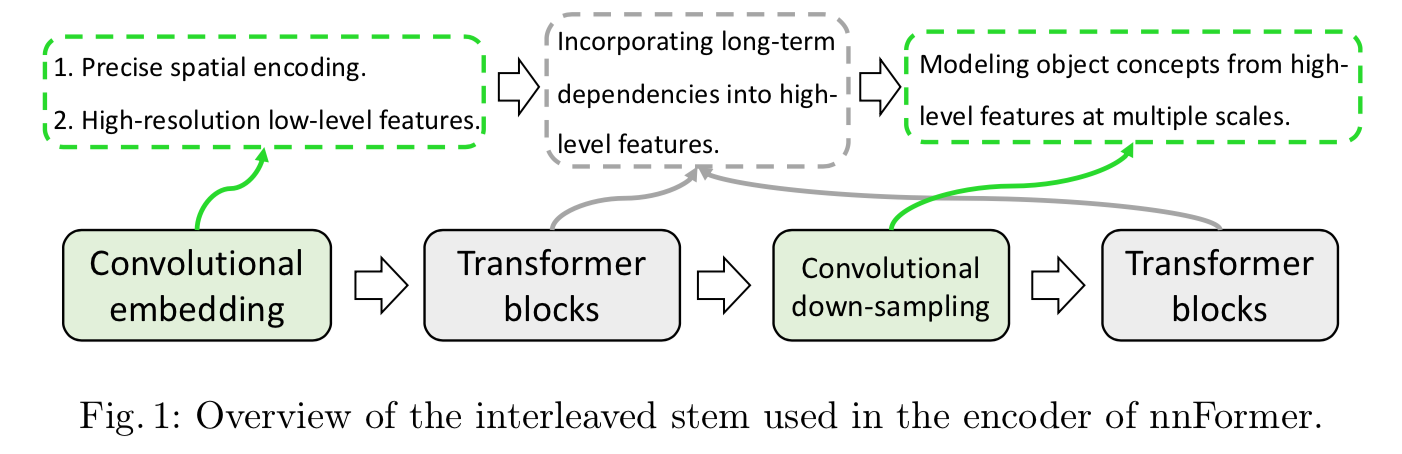
  - hybrid stem：卷积和self-attention都用上了，并且都能充分发挥能力，他的encoder：
    - 首先是一个轻量的conv embedding layer，好处是卷积能够提供更precise的spatial information，
    - 然后是交替的transformer blocks和convolutional down-sampling blocks，capture long-term dependencies at various scales
  - V-MSA：volume-based multi-head self-attention
    - a computational-efficient way to capture inter-slice dependencies
    - 计算复杂度降低90%以上
    - 应该就是类似于swin那种inter-patch & inter-patch吧？
方法
- overview
  - U-net结构：
    - embedding block + encoder + decoder + patch expanding block
    - 三次下采样 & 三次上采样
    - long residual connections
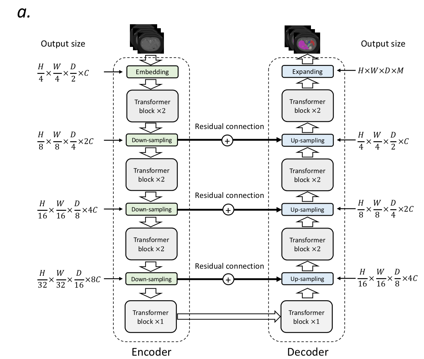
- encoder
  - input：3D patch $X \in R^{H \times W \times D}$
  - embedding block
    - 将3D patch转化成patch tokens，$X_e \in R^{\frac{H}{4}\frac{W}{4}\frac{D}{2}C}$，代表的是high-resolution spatial information
    - $\frac{H}{4}\frac{W}{4}\frac{D}{2}$是token个数
    - C是tensor channel，192/96
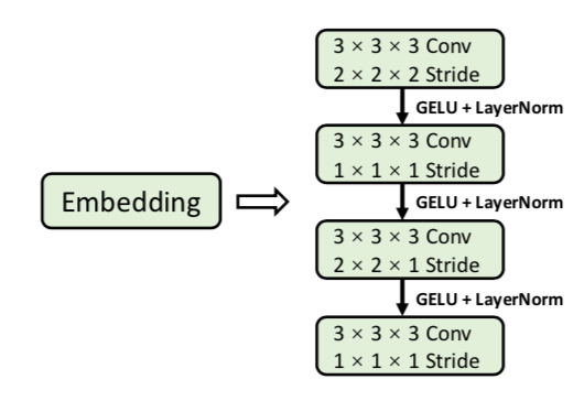
    - 4个连续的kernel3x3的卷积层替代Swin里面的big kernel：小卷积核给出的解释是计算量&感受野，没什么特别的，用卷积embedding给出的解释是pixel-level编码局部spatial信息，more precisely
    - 前三层卷积后面+GELU+LN，stride在1、3层，如图
  - transformer block
    - hierarchical
    - compute self-attention within 3D local volumes (instead of 2D local windows)
    - input：tokens representation of 3D patch， $X_t \in R^{L \times C}$
    - 首先reshape：对token sequence，再次划分local volume，$\tilde X_t \in R^{N_V \times N_T \times C}$
      - local volume里面包含一组空间相邻的tokens
      - $N_V$是volume的数目（类似Swin里面window的数目）
      - $N_T=S_H \times S_W \times S_D$ 是每个local volumes里面token的个数，{4,4,4}/{5,5,3}
    - 然后跟Swin一样，两个连续的transformer blocks，3D windows instead of 2D
      - V-MSA：volume-based multi-head self-attention
      - SV-MSA：shifted version
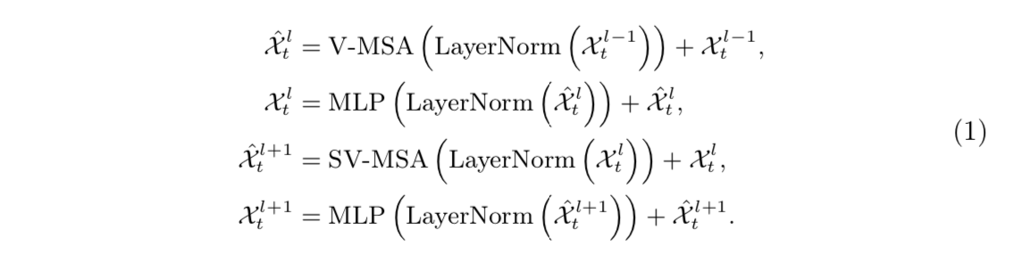
    - 反正就是3D版的swin，回去看swin更清晰
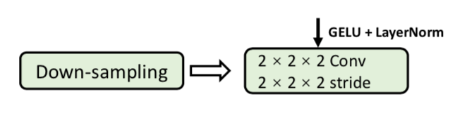
  - down-sampling block
    - 就是strided conv，说是相比较于neighboring concatenation，能产生更hierarchical的representation，有助于learn at multi scales
- decoder
  - 和encoder高度对称
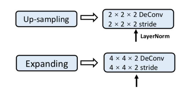
  - down-samp对标替换成strided deconvolution
  - 然后和encoder之间还有long-range connection，融合semantic和fine-grained information
  - 最后的expanding block也是用了deconv
实验

Swin-Unet: Unet-like Pure Transformer for Medical Image Segmentation

动机
- Unet-like pure Transformer
  - 用Swin transformer做encoder
  - 对称的decoder，用patch expanding layer做上采样
- outperforms full-convolution / combined methods
论点
- CNN的局限性
  - 提取explicit global & long-range information
  - meanwhile Swin在各项任务上SOTA了
- Swin-Unet
  - the first pure Transformer-based Unet-shaped architecture
  - consists of encoder, bottleneck, decoder and skip connections
  - token：non-overlapping patches split from the input image
  - fed into encoder：得到context features
  - fed into decoder：将global features再upsample回input resolution
  - patch expanding layer：不用conv/interpolation，实现spatial和feature-dim的increase
  - skip connection：对Transformer-based的Unet结构仍旧有效
方法
- overview
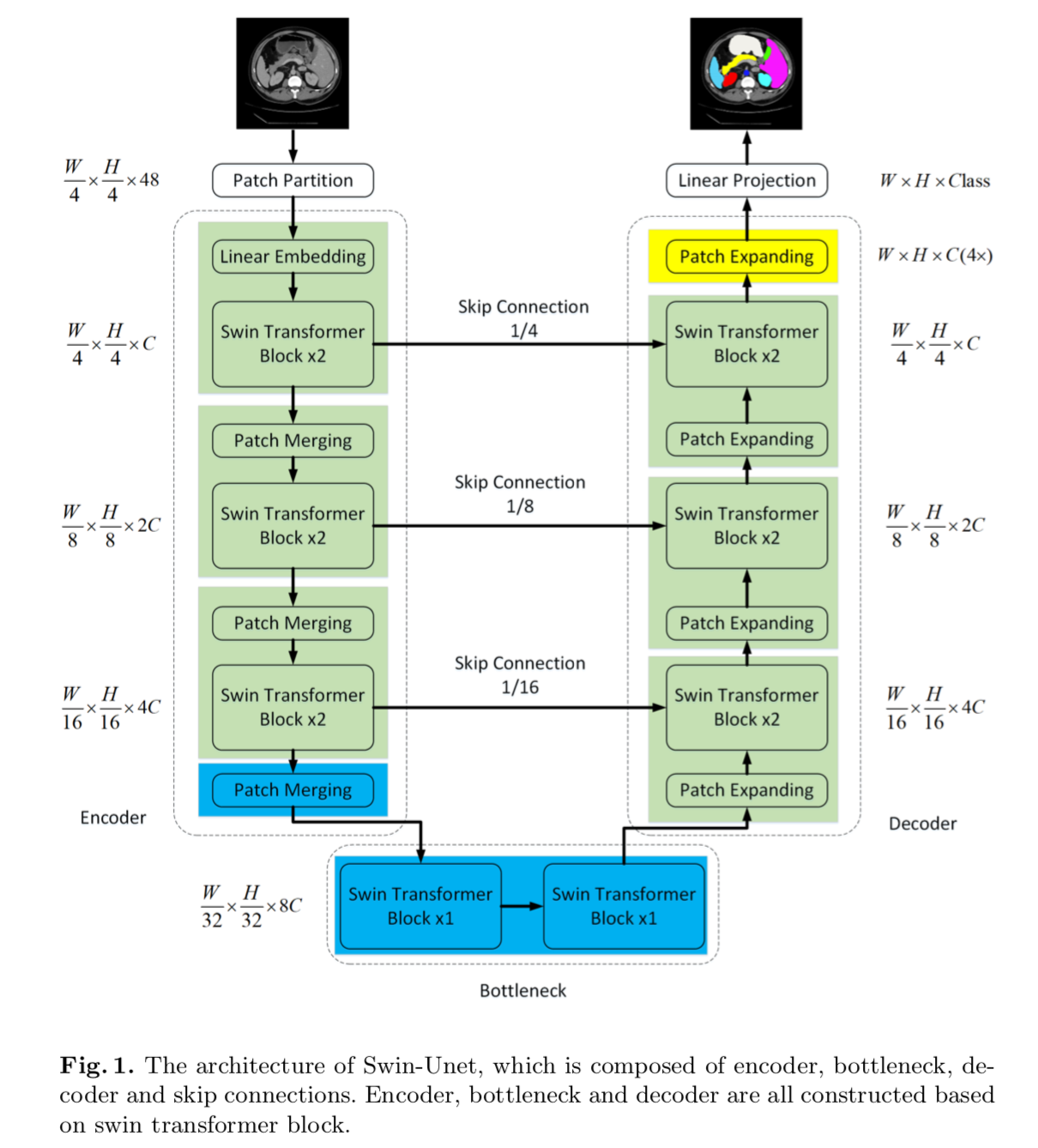
  - patch partition
    - 将图像切分成不重叠的patches，patch size是4x4
    - 每个patch的feature dimension就是4x4x3=48，也就是48-dim vec
  - linear embedding
    - 将固定的patch dimension映射到任意给定维度C
  - 交替的Swin Transformer blocks和Patch Merging
    - generate hierarchical feature representations
    - Swin Transformer block 是负责学feature representation的
    - Patch Merging是负责维度变换（下采样/上采样）的
  - 对称的decoder：交替的Swin Transformer blocks和Patch Expanding
    - Patch Expanding将相邻特征图拼接起来，组成2x大的特征图，同时减少特征维度
  - 最后一个Patch Expanding layer则执行4倍上采样
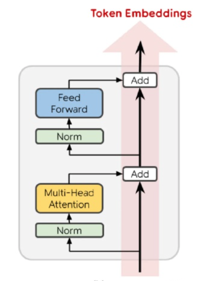
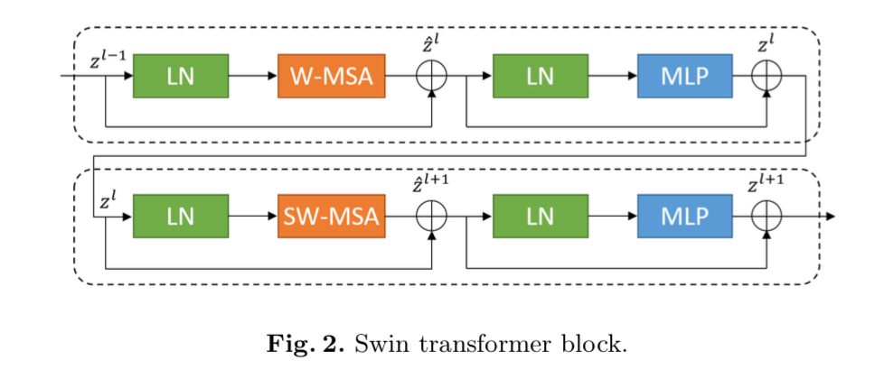
- Swin Transformer block
  - based on shifted windows
  - 两个连续的Transformer block为一组
  - 每个block内部都是LN-MSA-LN-MLP，residual，GELU
  - 第一个block的MSA是W-MSA
  - 第二个block的MSA是SW-MSA
- encoder
  - input：C-dim tokens，$\frac{H}{4} \times \frac{W}{4}$个tokens
  - patch merging layer
    - 将patches切分成2x2的4个parts
    - 然后将4个part在特征维度上concat
    - 然后接一个linear layer，将特征维度的dim转换为2C
    - 这样spatial resolution就downsampled by 2x
    - 特征维度加倍了2x
- bottleneck
  - encoder和decoder中间那个部分
  - 用了两个连续的Swin transformer block
  - 【QUESTION】也是shifited windows的吗？
  - 这个part特征维度不变
- decoder
  - patch expanding layer
    - given input features：$(\frac{W}{32} \times \frac{H}{32}\times 8C)$
    - 先是一个linear layer，加倍feature dim：$(\frac{W}{32} \times \frac{H}{32}\times 16C)$
    - 然后合并相邻4个patch tokens：$(\frac{W}{16} \times \frac{H}{16}\times 4C)$
- skip connection
  - concat以后接一个linear layer，保持特征维度不变
实验

UPerNet: Unified Perceptual Parsing for Scene Understanding

动机
- 人类对于图像的识别是存在多个层次的
  - scenes
  - objects inside
  - compositional parts
  - textures and surfaces
- our work
  - study a new task caled Unified Perceptual Parsing（UPP）：建立了一个“统一感知解析”的任务
  - 要求模型recognize as many visual concepts as possible
  - propose a multi-task framework UPerNet & a training strategy
- repo：https://github.com/CSAILVision/unifiedparsing
  - semantic segmentation
  - multi-task
论点
- various visual recognition tasks are mostly studied independently
  - 过去的task总是将不同level的视觉信息分开研究
  - is it possible for a neural network to solve several visual recognition tasks simultaneously?
- thus we propose Unified Perceptual Parsing（UPP）task
  - 有两个data issue
  - no single dataset annotated with all levels of visual information
  - 不同perceptual levels的标注形式也不统一
- thus we propose UPerNet
  - overcome the heterogeneity of different datasets
  - learns to detect various visual concepts jointly
  - 主要实现方式是每个iteration只选取一种数据集，同时只更新相关网络层
- we further propose a training method
  - enable the network to predict pixel-wise texture labels using only image-level annotations
方法
- Defining Unified Perceptual Parsing
  - 统一感知解析：从一张图中获取各种维度的视觉信息
    - scene labels
    - objects
    - parts of objects
    - materials and textures of objects
  - datasets
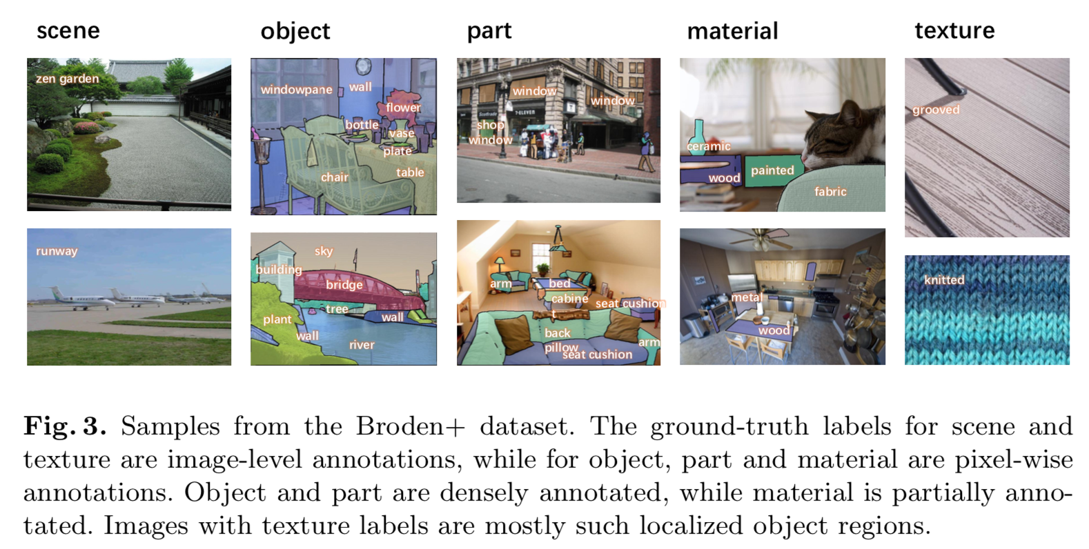
    - 使用了Broadly and Densely Labeled Dataset：整合了好几个数据集，contains various visual concepts
    - Objects, object parts and materials are segmented down to pixel level while textures and scenes are annotated
      
      at image level：目标、组成成分、材质是像素级标注，纹理和场景是图像级标注
    - standardize调整
      - data imabalance issue：丢掉一部分尾部数据
      - merge across dataset：合并不同数据集的同类数据
      - merge under-sampled labels：合并子类
    - our Broden+
      - 57, 095 images in total：51,617 training /5, 478 validation
      - 22, 210 images from ADE20K, 10, 103 images from Pascal-Context and Pascal-Part, 19, 142 images from Open- Surfaces and 5, 640 images from DTD
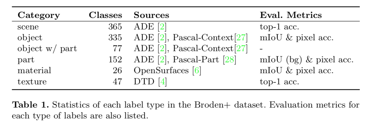
  - metrics
    - Pixel Accuracy (P.A.)：the proportion of correctly classified pixels
    - mean IoU (mIoU)：目标前景的平均IoU，会影响bg分割的表现
    - mIoU-bg：前景占比很小的时候，再加上bg IoU，object parts
    - top-1 acc：图像级标注使用top1 acc，scene and texture classification
- Designing Networks for Unified Perceptual Parsing
  - overview
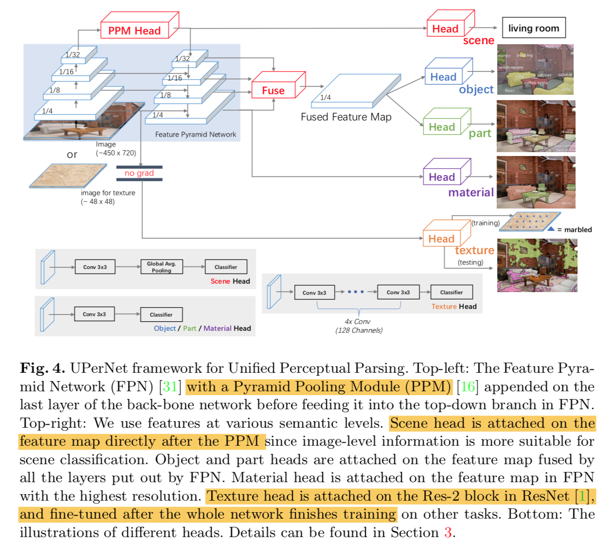
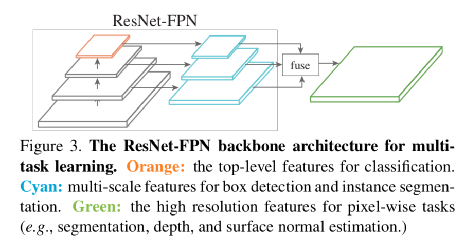
    - 因为包含high/low level visual tasks，所以网络也是multi-level的：FPN with a PPM
    - scene head是image-level classification label，直接接PPM的输出
    - object and part heads是多尺度的，使用FPN fusion的输出
    - material head是细粒度任务，使用FPN的highest resolution featuremap的输出
    - texture head是更加细粒度任务，接在backobne的Res-2 block后面，而且是在网络训练完其他任务以后再fine-tuning的
  - FPN
    - multi-level feature
    - use [top-down path + lateral connections] to fuse high-level semantic information into middle & low
    - conv-BN-ReLU，channel = 512
  - PPM
    - from PSPNet
    - 用来解决CNN理论上感受野足够大，但实际上相当小这个问题
    - 相比较于用dilated methods去扩大感受野的方式，好处是down-sampling rate更大（还是x32），能够提取high-level semantics
  - ResNet
    - 使用每个stage的输出作为level feature map，{C2, C3,C4,C5}，x4-x32
    - FPN的输出feature map，{P2, P3,P4,P5}，P5是PPM的输出
  - heads
    - scene head：分类器，接PPM输出，global average pooling + linear layer
    - object/parts head：实验发现使用fusion map表现好于P2，fusion map通过bilinear interpolating & concat & conv
    - materials head：on top of P2 rather than fused features
    - texture head：
      - texture label是图像级的，而且来自non-natural images
      - directly fusing these images with other natural images is harmful to other tasks
      - 同时我们希望预测是pixel-level
      - 我们把它接在C2上，append several convolutional layers，感受野small enough，而且backbone layers不回传梯度，只更新head layers
      - training images使用64x64的，确保模型只focus在local detail上
      - only fine-tune a few epochs
- training settings
  - poly learning rate，initial=0.2，power=0.9
  - weight decay=1e-4，momentum=0.9
  - training inputs：常用的目标检测rescale方法，随机将shorter side变成{300, 375, 450, 525, 600}
  - inference inputs：使用fixed shorter side 450
  - longer side < 1200
  - 为了防止noisy gradient，每个mini-batch随机选一种data source，按照数据集大小采样，只梯度更新相关path的参数
  - object and material segmentation计算前景loss
  - part segmentation计算前景+背景
  - on each GPU a mini-batch involves 2 images
  - sync-SGD & sync BN across 8 GPUs
  - training iterations of ADE20k (20k images) is 100k，其他数据集对应rescale
- Design discussion
  - previous segmentation networks主要是FCN，用pretrained backbones搭配dilated convs，扩大感受野的同时维持比较大的resolution
  - 但是原始的backobne，通常在stage4/5的时候有比较多的层，如resnet101的res4&res5就占了78层
    - 改用dilated convs一是计算量memory飙升
    - 二是有违最初的设计逻辑，未必还能发挥出原始的效能
    - 第三就是不好兼顾本文任务的classification task
实验

SegFormer: Simple and Efficient Design for Semantic Segmentation with Transformers

repo: https://github.com/NVlabs/SegFormer
动机
- propose a semantic segmentation framework SegFormer
  - simple, lightweight, efficient, powerful
  - hierarchical transformer + MLP decoder
- 特点
  - does not need positional encoding：在inference阶段切换图像分辨率不会引起性能变化
  - avoids complex decoders：MLP decoder主要就是merge multi levels
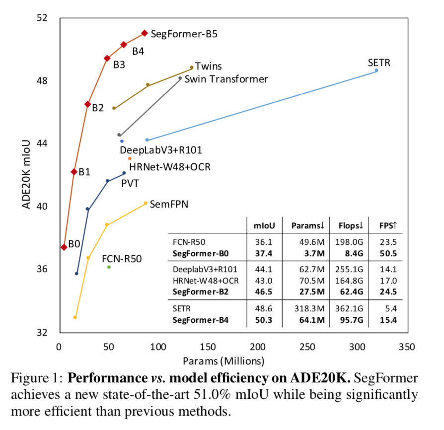
- scale up to obtain a family of models：SegFormer-B0 to SegFormer-B5
- verified on
  - SegFormer-B4：50.3% mIoU on ADE20K，SOTA
  - SegFormer-B5：84.0% mIoU on Cityscapes
论点
- SETR
  - ViT-back + several CNN decoders
  - ViT主要是计算量 & single-scale issue
  - 后续methods提出PVT、Swin、Twins等，主要focus在优化multi-scale的backbone，忽略了decoder的设计
- this paper （SegFormer）
  - redesigns both the encoder and the decoder
  - 改进的Transformer encoder：hierarchical & positional-encoding-free
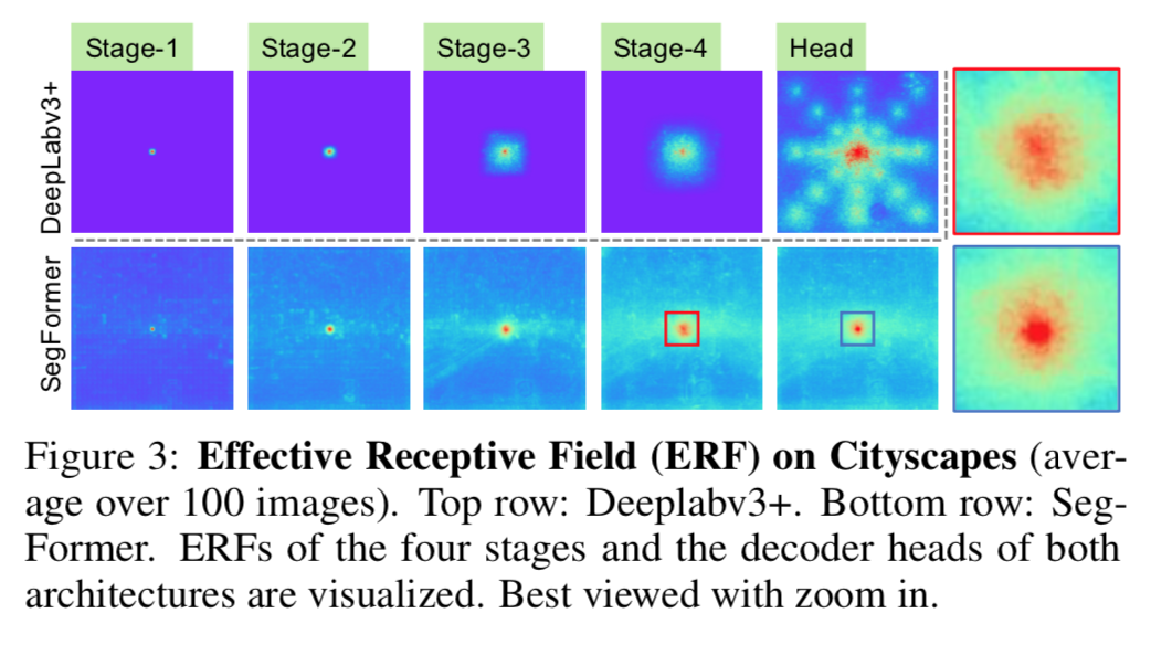
  - 设计的all-MLP decoder：lightweight but powerful，设计的核心思想是 to take advantage of the Transformer-induced features where the attentions of lower layers tend to stay local, whereas the ones of the highest layers are highly non-local
方法
- overview
  - encoder：
    - 使用了4x4的patch size，相比较于16x16的ViT，fine-grained patches is more preferred by semantic segmentation
    - multi-level features：x4，x8，x16，x32
  - decoder
    - 输入上述的multi-level features
    - 输出x4的segmentation mask
- Hierarchical Transformer Encoder
  - We design a series of Mix Transformer encoders (MiT)：MiT-B0 to MiT-B5
  - 基于PVT的efficient self-attention module
    - 针对原始attention block的平方时间复杂度
    - use a reduction ratio R to reduce the length of sequence K：注意是改变K的长度，而不是Q
    - given原始序列长度$N=HW$，feature dimensions $C$
      - 先reshape：$\hat K = Reshape(\frac{N}{R},CR)(K)$
      - 再降维：$K=Linear(CR,C)(\hat K)$
    - 计算量从O(N^2)下降到O(N^2/R)
    - set R to [64, 16, 4, 1] from stage-1 to stage-4
  - 同时提出了several novel designs
    - overlapped patch merging
      - 本文的一个论点是ViT用non-overlapping patches去做patch merging，相邻patch之间没有保留local continuity，所以需要positional encoding
      - 所以use an overlapping patch merging process
      - notations
        
        patch size K=7/3
        
        stride S=4/2
        
        padding size P=3/1 (valid padding)
        
        patch merging操作仍旧通过卷积来实现
    - positional-encoding-free design
      - ViT修改resolution要同步interpolatePE，还是会引起掉点
      - we introduce Mix-FFN
        
        在FFN中夹了一个conv3x3
        
        sufficient to provide positional information
        
        甚至可以用depth-wise convolutions节省参数量
      - we argure that adding PE is not necessary in semantic segmentation
- Lightweight All-MLP Decoder
  - idea是transformer有着远大于传统CNN的有效感受野，所以decoder可以轻量一点，不用再堆block
  - 4 main steps
    - unify：multi-level的feature maps各自通过MLP layer to unify the channel dimension
    - upsample：所有的features上采样到x4，biliear interp
    - fuse：concat + MLP(实际代码里用了1x1conv-bn-relu)
    - seg head：MLP，预测mask仍在x4尺度上
实验
- training settings
  - AdamW：lr=2e-4，weight decay=1e-4
  - poly LR：power=0.9，by iteration

GRAPH ATTENTION NETWORKS

发表于 2021-11-17 |

official repo: https://github.com/PetarV-/GAT

reference: https://zhuanlan.zhihu.com/p/34232818

归纳学习（Inductive Learning）：先从训练样本中学习到一定的模式，然后利用其对测试样本进行预测（即首先从特殊到一般，然后再从一般到特殊），这类模型如常见的贝叶斯模型。
转导学习（Transductive Learning）：先观察特定的训练样本，然后对特定的测试样本做出预测（从特殊到特殊），这类模型如k近邻、SVM等。

GRAPH ATTENTION NETWORKS

动机
- task：node classification
- 在GCN基础上引入 masked self-attentional layers
- specify different weights to different nodes in a neighborhood，感觉是用attention矩阵替换邻接矩阵？
论点
- the attention architecture properties
  - parallelizable，计算高效
  - can be applied to graph nodes having different degrees，这个邻接矩阵也可以啊
  - directly applicable to inductive learning problems，是说原始GCN那种semi-supervised场景吗
  - 感觉后面两点有点牵强
- GCN
  - 可以避免复杂的矩阵运算
  - 但是依赖固定图结构，不能直接用于其他图
methods
- graph attentional layer
  - input：node features
    - N个节点，F-dim representation
    - $h=\{\overrightarrow {h_1},\overrightarrow {h_2},…,\overrightarrow {h_N} \}$，$\overrightarrow {h_i} \in R^F$
  - output：a new set of node features
    - $h=\{\overrightarrow {h_1^{‘}},\overrightarrow {h_2^{‘}},…,\overrightarrow {h_N^{‘}} \}$，$\overrightarrow {h_i} \in R^{F^{‘}}$
  - a weight matrix
    - $W \in R^{F \times F^{‘}}$
    - applied to every node
  - then self-attention
    - compute attention coefficients：$e_{ij} = a(W\overrightarrow {h_i},W\overrightarrow {h_j})$
      - attention mechanism a：是一个single-layer feedforward neural network + LeakyReLU(0.2)
      - weight vector $\in R^{2F^{‘}}$
    - softmax norm
    - overall expression
      - 两个feature vector concat到一起
      - 然后全连接层+LeakyReLU
      - 然后softmax
    - 表达的是节点j对节点i的重要性
    - masked attention：inject graph structure，只计算节点i的neighborhood的importance
    - neighborhood：the first-order neighbors
    - 加权和 + nonlinearity
    - multi-head attention：
      - trainable weights有多组，一个节点与其neighborhood的attention coefficients有多组
      - 最后每组weights计算出那个new node feature（加权平均+nonlinear unit），可以选择concat/avg，作为最终输出
      - concat
      - 如果是网络最后一层的MHA layer，先avg，再非线性激活函数：
    - overall
  - comparisons to related work
    - our proposed GAT layer directly address several issues that were present in prior approaches
      - computationally efficient，说是比矩阵操作高效，这个不懂
      - assign different importance to nodes of a neighborhood，这个GCN with tranable adjacent matrix不也是一样性质的吗，不懂
      - enable 有向图
      - enable inductive learning，可以被直接用于解决归纳学习问题，即可以对从未见过的图结构进行处理，为啥可以不懂
    - 数学表达上看，attention和adjacent matrix本质上都是用来建模graph edges的
      - adj-trainable GCN：dag paper里面那种，adjacent matrix本身就是一个可训练变量(N,N)，随着训练更新参数
      - GAT：attention的更新引入了新的线性层权重 $ W \in R^{2F^{‘}}$

GPT

发表于 2021-10-27 |

GPT papers，openAI三部曲，通用预训练模型
- [2018 GPT-1] Improving Language Understanding by Generative Pre-Training：transformer-based，pre-training+task-specific finetuning，将所有的task的输入都整合成sequence-to-sequence form，结构上不需要task-specific architecture
- [2019 GPT-2] Language Models are Unsupervised Multitask Learners：对GPT-1结构上微调，引入huge dataset进行无监督训练
- [2020 GPT-3] Language models are few-shot learners：scaling up LMs，zero-shot
- BERT有3亿参数

GPT-1: Improving Language Understanding by Generative Pre-Training

动机
- NLP tasks
  - textual entailment：文本蕴含
  - question answering
  - semantic similarity assessment
  - document classification
- labeled data少，unlabeled corpora充足
- large gains can be realized by
  - generative pre-training of a language model on diverse unlabeled corpus，无监督general model，learn universal representations
  - discriminative fine-tuning on specific task，有监督task-specific model，adapt to wide range of tasks
- general task-agnostic model能够打败discriminatively trained models
- use task-aware input transformations
论点
- learn from raw text &alleviate the dependence on supervised learning still challenging：
  - 不清楚选什么optmization objectives：language modeling/machine translation/discourse coherence
  - effective way to transfer：加task-specific模型结构改动/auxiliary learning objectives/learning schemes
- two-stage training procedure
  - pretrain + fine-tuning
  - use Transformer：better handling long-term dependencies
  - task-specific input adaptions将输入处理成structured词向量序列
- evaluate on
  - natural language inference
  - question answering
  - semantic similarity
  - text classification
方法
- overview
  - architecture：transformer decoder
  - training objectives
    - unsupervised：text prediction，前文预测后文
    - supervised：task classifier，对整个序列分类
- Unsupervised pre-training
  - given unsupervised corpus of tokens $U={u_1, …, u_n}$
  - context window size $k$
  - use standard language modeling objective：$L_1(U)=\sum log P(u_i|u_{i-k},…,u_{i-1};\Theta)$
  - use multi-layer Transformer decoder
    - input：$h_0 = UW_e + W_p$
    - attention blocks：$h_l = tranformer_block(h_{l-1}), \forall l\in[1,n]$
    - output：$P(u)=softmax(h_l W_e^T)$
  - use SGD
- Supervised fine-tuning
  - given labeled dataset $C$ consists of $[x^1,…,x^m;y]$ instances
  - use the final transformer block’s activation $h_l^m$
  - fed into an linear+softmax output layer：$P(y|x^1,…,x^m)=softmax(h_l^mW_y)$
  - 优化目标是y：$L_2(C) = \sum log(P(y|x^1,…,x^m))$
  - 实验发现加上Unsupervised loss helps learning：提升泛化性，加速收敛
    $L_3(C) = L_2(C) + \lambda * L_1(C)$
- Task-specific input transformations
  - certain tasks has structured inputs如问答pairs/triplets
  - we convert them into ordered sequences
    - Textual entailment：将前提premise和推理hypothesis concat在一起
    - Similarity tasks：两个文本没有先后顺序关系，所以一对文本变成顺序交换的两个sequence，最后的hidden units $h^m_l$相加，然后接输出层
    - Question Answering and Commonsense Reasoning：given document $z$, question $q$, and possible answers $\{a_k\}$，context $zq$和每个答案$a_i$都构造一组连接，然后分别independently processed with our model，最后共同接入一个softmax，生成对所有possible answers的概率分布
  - 所有的连接都使用分隔符$
  - 所有的sequence的首尾都加上一个randomly initialized start&end tokens
实验

GPT-2: Language Models are Unsupervised Multitask Learners

动机
- more general models which can perform many tasks
- train language model
  - without explicit supervision
  - trained on a new dataset of millions of webpages called WebText
  - outperforms several baselines
- GPT-2：a 1.5B parameter Transformer
论点
- Machine learning systems are sensitive to slight changes of
  - data distribution
  - task specification
  - ‘narrow experts’
  - lack of generalization since ingle task training on single domain datasets
- methods
  - multitask training：还不成熟
  - pretraining + finetuning：still require supervised training
- this paper
  - connect the two lines above
  - perform donw-stream tasks in a zero-shot setting
方法
- natural sequential characteristic makes the general formulation $p(output|input)$
  $p(x) = \Pi_{i=1}^n p(s_{n-k}, ..., s_n|s_1, ..., s_{n-k-1})$
- task specific system requires the probabilistic framework also condition on the task to be performed $p(output|input, task)$
  - architectural level：task-specific encoders/decoders
  - algorithmic level：like MAML
  - or in a more flexible way to specify tasks：write all as sequences
    - translation：(translate to french, english text, french text)
    - comprehension：(answer the question, document, question, answer)
- training dataset
  - 海量document可以通过爬虫获得but significant data quality issues
  - 与target dataset similar的外部doc的子集能够给到提升
  - 因此本文设定了一个搜集文本的机制：Reddit的外链，去掉Wikipedia
- input representation
  - word-level language model VS byte-level language model
    - word-level performs better
    - 但是受到vocabulary限制
  - Byte Pair Encoding (BPE)
    - combine the empirical benefits of word-level LMs with the generality of byte-level approaches
    - 具体改进还没理解
- model
  - Transformer-based，few modifications on GPT-1 model
    - layer normalization was moved to the input of each sub-block
    - additional layer normalization was added after the final self-attention block
    - initialization on residual path：N个residual layers，就将residual weights rescale $\frac{1}{\sqrt{N}}$
    - context size：1024
    - batch size：512
  - residual block
实验

GPT-3: Language Models are Few-Shot Learners

动机
- zero-shot：pretraining+finetuning scheme还是需要task-specific finetuning datset
- scale-up：scaling up language models greatly improves general few-shot performance

dag

发表于 2021-10-11 |

美研院的论文，检测，用于腰椎/髋关节关键点提取
preparations
1. hrnet
2. pspModule

Structured Landmark Detection via Topology-Adapting Deep Graph Learning

动机
- landmark detection
  - 特征点检测
  - identify the locations of predefined fiducial points
  - capture relationships among 解剖学特征点
- 一个难点：遮挡/复杂前景状态下，landmark的准确检测和定位——structual information
- the proposed method
  - 用于facial and medical landmark detection
  - topology-adapting：learnable connectivity
  - learn end-to-end with two GCNs
论点
- heatmap regression based methods
  - 将landmarks建模成heatmaps，然后回归
  - lacking a global representation
  - 核心要素有bottom-up/top-down paths & multi-scale fusions & high resolution heatmap outputs
- coordinate regression based methods
  - potentially incorporate structural knowledge but a lot yet to be explored
  - falls behind heatmap-based ones
  - 核心要素是cascaded & global & local
  - 好处是结构化，不丢点，不多点，但是不一定准
- graph methods
  - 基于landmark locations和landmark-to-landmark-relationships构建图结构
  - most methods relies on heatmap detection results
  - we would directly regress landmark locations from raw input image
- we propose
  - DAG：deep adaptive graph
  - 将landmarks建模成graph图
  - employ global-to-local cascaded Graph Convolution Networks逐渐将landmark聚焦在目标位置
  - graph signals combines
    - local image features
    - graph shape features
  - cascade
    - two GCNs
    - 第一个预测一个global transform
    - 第二个预测local offsets to further adjust
  - contributions
    - effectively exploit the structural knowledge
    - allow rich exchange among landmarks
    - narrow the gap between coordinate & heatmap based methods
方法
- the cascaded-regression framework
  - input
    - image
    - initial landmarks from the mean shape
  - outputs
    - predicted landmark coordinates in multiple steps
  - feature
    - use graph representation
    - G = (V,E,F)
      - V是节点，代表landmarks，也就是特征点，表示为(x,y)的坐标
      - E是边，代表connectivity between landmarks，表示为(id_i, id_k)的无向/有向映射，整体的E matrix是个稀疏矩阵
      - F是graph signals，capturing appearance and shape information，表示为高维向量，如256-dim vec，与节点V一一对应，用于储存节点信息，在GCN中实际进行计算交互
  - overview
    - summary
      - cascade：一个GCN-global做粗定位，迭代多个GCN-local做precise定位
      - interpolation：feature map到feature nodes的转换，通过interpolation，【是global interp吗，是基于initial mean coords吗】
      - regression：【targets的具体坐标表示？？？】
      - inital graph：训练集的平均值
      - graph signal：visual feature和shape feature
- Cascaded GCNs
  - GCN-global：global transformation
  - GCN-local：coordinate offsets
  - share the same GCN architecture
  - graph convolution
    - 核心思想就是：给定一个图结构（with connectivity E），每一次堆叠graph convolution，就是在对每个图节点，基于其自身$f_k^i$和邻居节点$f_k^j$的当前graph feature，weighted aggregating，结果作为这个节点这次图卷积的输出$f_{k+1}^i$
      $f_{k+1}^i = W_1 f_k^i + \sum_j e_{ij}W_2 f_k^j$
    - learnable weight matrices $W_1$ 和 $W_2$
    - 可以看作是邻居节点间信息交互的一种方式
  - Global Transformation GCN
    - 这个model的作用是将initial landmarks变换到coarse targets
    - 参照STN，
      - recall STN
      - 使用perspective transformation透视变换，引入9个scalars，进行图形变
    - workflow
      - given a target image
      - initialize landmark locations $V^0$ using trainingset mean
      - GCN-global + GIN 预测perspective transformation
      - 进而得到变换后的节点位置
    - graph isomorphism network (GIN)
      - 图的线性层
      - 输入是GCN-global的graph features $\{f_k^i\}$
      - 输出是9-dim vector
      - 计算方式
        
        READOUT：sum the features from all nodes
        
        CONCAT：得到一个高维向量
        
        MLP：9-dim fc
        
        最后得到9-dim的perspective transformation scalar
    - coordinate update
      - 将9-dim $f^G$ reshape成3x3 transformation matrix M
      - 然后在当前的landmark locations $V^0$上施加变换——矩阵左乘
  - Local Refinement GCN
    - GCN结构与global的一致，但是不share权重
    - 最后的GIN头变了
      - 输出改成2-dim vector
      - represents coordinate offsets
    - coordinate update
      - 加法，分别在x/y轴坐标上
    - we perform T=3 iterations
- Graph signal with appearance and shape information
  - Visual Feature
    - denote CNN输出的feature map H with D channels
    - encoding整个feature map：bi-linear interpolation at the landmark location $v_i$，记作$p_i$，是个D-dim vector
  - Shape Feature
    - visual feature对节点间关系的建模，基于global map全局信息提取，比较隐式、间接
    - 事实上图结构能够直接对global landmarks shape进行encoding
    - 本文用displacement vectors，就是距离，每个节点的displacement vector记作$q_i=\{v_j-v_i\}_{j!=i}$，flatten成一维，对有N个节点的图，每个节点的q-vec维度为2*(N-1)
    - shape feature保存了structural information，当人脸的嘴被遮住的情况下，基于眼睛和鼻子以及结构性信息，就能够推断嘴的位置，这是Visual Feature不能直接表达的
  - graph signal
    - concat
    - result in a feature vector $f_i \in R^{D+2(N-1)}$
- Landmark graph with learnable connectivity
  - 大多数方法的图基于先验知识构建
  - we learn task-specific graph connectivity during training phase
  - 图的connectivity serves as a gate，用邻接矩阵表示，并将其作为learnable weights
- training
  - GCN-global
    - margin loss
    - $v_i^1$是GCN-global的预测节点坐标
    - m是margin
    - $[u]_+$是$max(0,u)$
    - push节点坐标到比较接近ground truth就停止了，防止不稳定
  - GCN-local
    - L1 loss
    - $v_i^T$是第T个iteration GCN-local的预测节点坐标
  - overall loss
    - 加权和
网络结构
- GCN-global
  - 三层basic graph convolution layer with residual（id path）
  - concat distance vector
  - 一层basic graph convolution
  - mean axis1（node axis）
  - fc，输出9-dim scalar，(b,9)
- GCN-local
  - 三层basic graph convolution layer with residual（id path）
  - relu
  - concat distance vector
  - 一层basic graph convolution
  - fc，输出2-dim coords for each node，(b,24,2)

KL Divergence

发表于 2021-09-27 |

KL divergence用于度量两个分布P和Q的差异，这种度量【不具有】对称性
- P是实际分布（pred probs）
- Q是建模分布（gt）
- $D_{KL}(P||Q)=\sum_i P(i)ln\frac{P(i)}{Q(i)}$
- 散度定义为分布P和分布Q之间的对数差异的加权和，用P的概率去加权
- 当Q是one-hot label的时候，要先clip再log
方法
- torch.nn.functional.kl_div(input, target, size_average=None, reduce=None, reduction=’mean’)
  - input：对数概率
  - target：概率
- tf.distributions.kl_divergence(distribution_a, distribution_b, allow_nan_stats=True, name=None)
  - distribution_a&b 来自tf.distributions.Categorical(logits=None, prob=None, …)
  - 传入logits/probs，先转换成distribution，再计算kl divergence
- torch.nn.KLDivLoss
- tf.keras.losses.KLDivergence
- tf.keras.losses.kullback_leibler_divergence
code

# torch version
import torch.nn as nn
import torch.nn.functional as F

class KL(nn.Module):
  	def __init__(self, args):
      	super(KL, self).__init__()
        self.T = args.temperature
        
		def forward(self, logits_p, logits_q):
      	log_p = F.log_softmax(logits_p/self.T, dim=1)
        q = F.softmax(logits_q/self.T, dim=1)
        loss = F.kl_div(log_p, p_t)

        
# keras version
import tensorflow as tf
import keras.backend as K

def kl_div(logits_p, logits_q):
  	T = 4.
    log_p = tf.nn.log_softmax(logits_p/T)      # (b,cls)
    log_q = tf.nn.log_softmax(logits_q/T)
    p = K.exp(log_p)
    return K.sum(p*(log_p-log_q), axis=-1)   # (b,)

Self-Knowledge Distillation

发表于 2021-09-17 |

动机
- 传统的知识蒸馏
  - by stage：先训练庞大的teacher
- self knowledge distillation
  - without the pretrained network
  - 分为data augmentation based approach 和 auxiliary network based approach
  - data augmentation approach如UDA，通过监督原始图像和增强图像的一致性，但是会loose local information，对pixel-level tasks不友好，而且监督信息是从logits层，没有直接去refine feature maps
- our approach FRSKD
  - auxiliary network based approach
  - utilize both soft label and featuremap distillation
论点
- various distillation methods
  - a是传统知识蒸馏，深绿色是pretrained teacher，浅绿色是student，橙色箭头是feature蒸馏，绿色箭头是soft label蒸馏
  - b是data augmentation based 自蒸馏，shared 网络，原图和增强后的图，用soft logits来蒸馏
  - c是auxiliary classifier based 自蒸馏，cascaded分类头，每个分类器都接前一个的
  - d是本文自蒸馏，和c最大的不同是bifpn结构使得两个分类器每个level的特征图之间都有连结，监督方式一样的
- FPN
  - PANet：上行+下行
  - biFPN：上行+下行+同层级联
方法
- overview
  - notations
    - dataset $D=\{(x_1,y_1), (x_2,y_2),…, (x_N,y_N)\}$
    - feature map $F_{i,j}$，i-th sample，j-th block
    - channel dimension $c_j$，j-th block
- self-teacher network
  - self-teacher network的目的是提供refined feature map和soft labels作为监督信息
  - inputs：feature maps $F_1, F_2, …, F_n$，也就是说teacher在进行梯度回传的时候到F就停止了，不会更新student model的参数
  - modified biFPN
    - 第一个不同：别的FPN都是在fuse之前先用一个fixed-dim 1x1 conv将所有level的feature map转换成相同通道数（如256），we design $d_i$ according to $c_i$，引入一个宽度系数width，$d_i=width*c_i$，
    - 第二个不同：使用depth-wise convolution
    - notations
      - BiFPN：每层dim固定的版本
      - BiFPNc：每层dim随输入变化的版本
- self-feature distillation
  - feature distillation
    - adapt attention transfer
    - 对feature map先进行channel-wise的pooling，然后L2 norm，提取spatial information
  - soft label distillation
    - 两个分类头的KL divergence
  - CE with gt
    - 两个分类头分别还有正常的CE loss
  - overall
    - 总的loss是4个loss相加：$L_{FRSKD}(x,y,\theta_c, \theta_t, K)=L_{CE}(x,y,\theta_c)+L_{CE}(x,y,\theta_t)+\alpha L_{KD}(x,\theta_c,\theta_t, K) + \beta L_{F}(T,F,\theta_c,\theta_T)$
    - $\alpha \in [1,2,3]$
    - $\beta \in [100,200]$
    - 【QUESTION】FRSKD updates the parameters by the distillation loss，$L_{KD}$ and $L_F$，which is only applied to the student network，这个啥意思暂时没理解
实验
- experiment settings
  - FRSKD\F：只做soft label的监督，不做feature map的监督
  - FRSKD：标准的本文方法
  - FRSKD+SLA：本文方法的基础上attach data augmentation based distillation

L2 Regularization and Batch Norm

发表于 2021-09-16 |

reference：

https://blog.janestreet.com/l2-regularization-and-batch-norm/

https://zhuanlan.zhihu.com/p/56142484

https://vitalab.github.io/article/2020/01/24/L2-reg-vs-BN.html

解释了之前的一个疑点：

在keras自定义的BN层中，没有类似kernel_regularizer这样的参数
在我们写自定义optmizer的时候，BN层也不进行weight decay的

L2 Regularization versus Batch and Weight Normalization

动机
- 两个common tricks：Normalization（BN、WN、LN等）和L2 Regularization
  - 发现两者结合时L2 regularization对normalization层没有正则效果
  - L2 regularization反而对norm layer的scale有影响，间接影响了learning rate
  - 现代优化器如Adam只能间接消除这种影响
论点
- BN
  - popular in training deep networks
  - solve the problem of covariate shift
  - 使得每个神经元的输入保持normal分布，加速训练
  - mean & variance：training time基于每个mini-batch计算，test time使用所有iteration的mean & variance的EMA
- usually trained with SGD with L2 regularization
  - result in weight decay：从数学表示上等价于对权重做衰减
  - 每一步权重scaled by a 小于1的数
  - 但是normalization strategies是对scale of the weights invariant的，因为在输入神经元之前都会进行norm
  - therefore
    - there is no regularizing effect
    - rather strongly influence the learning rate??👂
L2 Regularization
- formulation：
  - 在loss的基础上加一个regularization term，$L_{\lambda}(w)=L(w)+\lambda ||w||^2_2$
  - loss是每个样本经过一系列权重运算，$L(w)=\sum_N l_i (y(X_i;w,\gamma,\beta))$
  - 当使用normalization layer的时候：$y(X_i;w,\alpha,\beta)=y(X_i;\alpha w,\gamma,\beta)$，即loss term不会变
  - $L_{\lambda}(\alpha w)=L(w)+\lambda||w||^2_2$
  - 在有normalization layer的时候，L2 penalty还是能够通过reg term force权重的scale越来越小，但是不会影响优化进程（不影响main objective value），因为loss term不变
- Effect of the Scale of Weights on Learning Rate
  - BN层的输出是scale invariant的，但是梯度不是，梯度是成反比被抑制的！
  - 所以weights在变小，同时梯度在变大！
  - 在减小weight scale的时候，网络的梯度会变大，等价于学习率在变大，会引起震荡不稳定
  - 所以在设定hyper的时候，如果我们要适当加大weight decay $\lambda$，就要反比scale学习率
- Effect of Regularization on the Scale of Weights
  - during training the scale of weights will change
    - the gradients of the loss function will cause the norm of the weights to grow
    - the regularization term causes the weights to shrink

SAM loss

发表于 2021-09-10 |

google brain，引用量51，但是ImageNet榜单/SOTA模型的对比实验里面经常能够看到这个SAM，出圈形式为分类模型+SAM

SAM：Sharpness-Aware Minimization，锐度感知最小化

official repo：https://github.com/google-research/sam

Sharpness-Aware Minimization for Efficiently Improving Generalization

动机
- heavily overparametered models：training loss能训到极小，但是generalization issue
- we propose
  - Sharpness-Aware Minimization (SAM)
  - 同时最小化loss和loss sharpness
  - improve model generalization
  - robustness to label noise
- verified on
  - CIFAR 10&100
  - ImageNet
  - finetuning tasks
论点
- typical loss & optimizer
  - population loss：我们实际想得到的是在当前训练集所代表的分布下的最优解
  - training set loss：但事实上我们只能用所有的训练样本来代表这个分布
  - 因为loss函数是non-convex的，所以可能存在多个local even global minima对应的loss value是一样的，但是generalization performance确是不同的
- 成熟的全套防止过拟合手段
  - loss
  - optimizer
  - dropout
  - batch normalization
  - mixed sample augmentations
- our approach
  - directly leverage the geometry of the loss landscape
  - and its connection to generalization (generalization bound)
  - proved additive to existing techniques
方法
- motivation
  - rather than 寻找一个weight value that have low loss，我们寻找的是那种连带他临近的value都能有low loss的value
  - 也就是既有low loss又有low曲度
- sharpness term
  - $\max \limits_{||\epsilon||_p < \rho} L_s(w+\epsilon) - L_s(w)$
  - 衡量模型在w处的sharpness
- Sharpness-Aware Minimization (SAM) formulation
  - sharpness term再加上train loss再加上regularization term
  - $L_S^{SAM}(w)=\max\limits_{a} L_s(w+\epsilon)$
  - $\min \limits_{w} L_S^{SAM}(w) + \lambda ||w||^2_2$
  - prevent the model from converting to a sharp minimum
- effective approximation
  - bound
    - with $\frac{1}{p} + \frac{1}{q} = 1$
  - approximation
- pseudo code
  - given a min-batch
  - 首先计算当前batch的training loss，和当前梯度，$w_t$ to $w_{t+1}$
  - 然后计算近似为梯度norm的步长$\hat\epsilon(w)$，equation2，$w_t$ to $w_{adv}$，这里面的adv联动了另一篇论文《AdvProp: Adversarial Examples Improve Image Recognition》
  - 然后计算近似的sharpness term，可以理解为training loss在w邻居处的梯度，equation3，应该是蓝色箭头的反方向，图上没标记出来
  - 用w邻居的梯度来更新w的权重，用负梯度（蓝色箭头）
  - overll就是：要向前走之前，先回退，缺点是两次梯度计算，时间double
实验结论
- 能优化到损失的最平坦的最小值的地方，增强泛化能力

MuST谷歌多任务自训练

发表于 2021-09-01 |

recollect

[SimCLR]

[MoCo]

Multi-Task Self-Training for Learning General Representations

动机
- learning general feature representations
- expect a single general model
  - 相比较于training specialized models for various tasks
  - harness from independent specialized teacher models
  - with a multi-task pseudo dataset
  - trained with multi-task learning
- evalutate on 6 vision tasks
  - image recognition (classification, detection, segmentation)
  - 3D geometry estimation
论点
- pretraining & transfer learning
  - transformer一般都是这个套路，BiT&ViT
  - pretraining
    - supervised / unsupervised
    - learn feature representations
  - transfer learning
    - on downstream tasks
    - the features may not necessarily be useful
    - 最典型的就是ImageNet pre-training并不能improve COCO segmentation，但是Objects365能够大幅提升
  - pretraining tasks必须要和downstream task align，learn specialized features，不然白费
- learning general features
  - a model simultaneously do well on multiple tasks
  - NLP的bert是一个典型用多任务提升general ability的
  - CV比较难这样做是因为标签variety，没有这样的大型multi-task dataset
- multi-task learning
  - shared backbone (如ResNet-FPN)
  - small task-specific heads
- self-training
  - use a supervised model to generate pseudo labels on unlabeled data
  - then a student model is trained on the pseudo labeled data
  - 在各类任务上都proved涨点
  - 但是迄今为止都是focused on a single task
- in this work
  - lack of large scale multi-task dataset的issue，通过self-training to fix，用pseudo label
  - specialized/general issue，通过多任务，训练目标就是六边形战士，absorb the knowledge of different tasks in the shared backbone
  - three steps
    - trains specialized teachers independently on labeled datasets （分类、分割、检测、深度估计）
    - the specialized teachers are then used to label a larger unlabeled dataset（ImageNet） to create a multi- task pseudo labeled dataset
    - train a student model with multi-task learning
  - MuST的特质
    - improve with more unlabeled data，数据越多general feature越好
    - can improve upon already strong checkpoints，在海量监督高精度模型基础上fine-tune，仍旧能在downstream tasks涨点
方法
- Specialized Teacher Models
  - 4 teacher models
    - classification：train from scratch，ImageNet
    - detection：train from scratch，Object365
    - segmentation：train from scratch，COCO
    - depth estimation：fine-tuning from pre-trained checkpoint
  - pseudo labeling
    - unlabeled / partially labeled datasets
    - for detection：hard score threshold of 0.5
    - for segmentation：hard score threshold of 0.5
    - for classification：soft labels——probs distribution
    - for depth：直接用
- Multi-Task Student Model
  - 模型结构
    - shared back
      - C5：for classification
      - feature pyramids {P3,P4,P5,P6,P7}：for detection
      - fused P2：for pixel-wise prediction，把feature pyramids rescale到level2然后sum
    - heads
      - classification head：ResNet design，GAP C5 + 线性层
      - object detection task：Mask R-CNN design，RPN是2 hidden convs，Fast R-CNN是4 hidden convs + 1 fc
      - pixel-wise prediction heads：3 hiddent convs + 1 linear conv head，分割和深度估计任务independent，不share heads
  - Teacher-student training
    - using the same architecture
    - same data augmentation
    - teacher和student的main difference就是dataset和labels
  - Learning From Multiple Teachers
    - every image has supervision for all tasks
    - labels may come from supervised or pseudo labels
    - 如果使用ImageNet数据集，classification就是真标签，det/seg/depth supervision则是伪标签
    - balance the loss contribution
      - 加权和，task-specific weights
      - for ImageNet，use $w_i = \frac{b_slr_{it}}{b_{it}lr_{s}}$
      - follow the scaling rule：lr和batch size成正比
      - except for depth loss
  - Cross Dataset Training
    - training across ImageNet, object365 and COCO
    - 有标签的就用原标签，没有的用伪标签，supervised labels and pseudo labels are treated equally，而不是分别采样和训练
    - balance the datasets：合在一起然后均匀采样
  - Transfer Learning
    - 得到general student model以后，fine-tune on 一系列downstream tasks
    - 这些downstream datasets与MuST model的训练数据都是not align的
    - 这个实验要证明的是supervised model（如teacher model）和self-supervised model（如用pseudo label训练出来的student model），在downstream tasks上迁移学习能performance是差不多的，【注意⚠️：如果迁移datasets前后align就不是这样了，pretrain显然会更好！！！】

GHM

发表于 2021-08-31 |

families:

[class-imbalanced CE]
[focal loss]
[generalized focal loss] focal loss(CE)的连续版本
[ohem]

keras implementation:

def weightedCE_loss(y_true, y_pred):
		alpha = .8
		pt = K.abs(y_true-y_pred)
		# clip
    pt = K.clip(pt, K.epsilon(), 1-K.epsilon())
    # ce
    ce = -K.log(1.-pt)
    # pos/neg reweight
    wce = tf.where(y_true>0.5, alpha* , (1-alpha)* )
    return wce

def focal_loss(y_true, y_pred):
		alpha = .25
		gamma = 2
		
		pt = K.abs(y_true-y_pred)
		# clip
    pt = K.clip(pt, K.epsilon(), 1-K.epsilon())
    # easy/hard reweight
		fl = -K.pow(pt, gamma) * K.log(1.-pt)
    # pos/neg reweight
    fl = tf.where(y_true>0.5, alpha*fl, (1-alpha)*fl)
    return fl
  
 def generalized_focal_loss(y_true, y_pred):
		# CE = -ytlog(yp)-(1-yt)log(1-yp)
  	# GFL = |yt-yp|^beta * CE
    beta = 2
    # clip y_pred
    y_pred = K.clip(y_pred, K.epsilon(), 1-K.epsilon())
    # ce
    ce = -y_true*K.log(y_pred) - (1-y_true)*K.log(1-y_pred)   # [N,C]
    # easy/hard reweight
    gfl = K.pow(K.abs(y_true-y_pred), beta) * ce
    return gfl

def ce_ohem(y_true, y_pred):
  	pt = K.abs(y_true-y_pred)
		# clip
    pt = K.clip(pt, K.epsilon(), 1-K.epsilon())
    # ce
    ce = -K.log(1.-pt)
    # sort loss
    k = 50
    ohem_loss, indices = tf.nn.top_k(ce, k=k)   # topk loss: [k,], topk indices: [k,], idx among 0-b
    mask = tf.where(ce>=ohem_loss[k-1], tf.ones_like(ce), tf.zeros_like(ce))
    return mask*ce

Gradient Harmonized Single-stage Detector

动机
- one-stage detector
  - 核心challenge就是imbalance issue
  - imbalance between positives and negatives
  - imbalance between easy and hard examples
  - 这两项都能归结为对梯度的作用：a term of the gradient
- we propose a novel gradient harmonizing mechanism (GHM)
  - balance the gradient flow
  - easy to embed in cls/reg losses like CE/smoothL1
  - GHM-C for anchor classification
  - GHM-R for bounding box refinement
- proved substantial improvement on COCO
  - 41.6 mAP
  - surpass FL by 0.8
论点
- imbalance issue
  - easy and hard：
    - OHEM
    - directly abandon examples
    - 导致训练不充分
  - positive and negative
    - focal loss
    - 有两个超参，跟data distribution绑定
    - not adaptive
  - 通常正样本既是少量样本又是困难样本，而且可以通通归结为梯度分布不均匀的问题
    - 大量样本只贡献很小的梯度，通常对应着大量负样本，总量多了也可能会引导梯度（左图）
    - hard样本要比medium样本数量大，我们通常将其看作离群点，因为模型稳定以后这些hard examples仍旧存在，他们会影响模型稳定性（左图）
    - GHM的目标就是希望不同样本的gradient contribution保持harmony，相比较于CE和FL，简单样本和outlier的total contribution都被downweight，比较harmony（右图）
- we propose gradient harmonizing mechanism (GHM)
  - 希望不同样本的gradient contribution保持harmony
  - 首先研究gradient density，按照梯度聚类样本，并相应reweight
  - 针对分类和回归设计GHM-C loss和GHM-R loss
  - verified on COCO
    - GHM-C比CE好得多，sligtly better than FL
    - GHM-R也比smoothL1好
    - attains SOTA
  - dynamic loss：adapt to each batch
方法
- Problem Description
  - define gradient norm $g = |p - p^*|$
  - the distribution g from a converged model
    - easy样本非常多，不在一个数量级，会主导global gradient
    - 即使收敛模型也无法handle一些极难样本，这些样本梯度与其他样本差异较大，数量还不少，也会误导模型
- Gradient Density
  - define gradient density $GD(g) = \frac{1}{l_{\epsilon}(g)} \sum_{k=1} \delta_{\epsilon}(g_k,g)$
    - given a gradient value g
    - 统计落在中心value为$g$，带宽为$\epsilon$的范围内的梯度的样本量
    - 再用带宽去norm
  - define the gradient density harmony parameter $\beta_i = \frac{N}{GD(g_i)}$
    - N是总样本量
    - 其实就是与density成反比
    - large density对应样本会被downweight
- GHM-C Loss
  - 将harmony param作为loss weight，加入现有loss
  - - 可以看到FL主要压简单样本（基于sample loss），GHM两头压（基于sample density）
    - 最终harmonize the total gradient contribution of different density group
    - dynamic wrt mini-batch：使得训练更加efficient和robust
  - Unit Region Approximation
    - 将gradient norm [0,1]分解成M个unit region
    - 每个region的宽度$\epsilon = \frac{1}{M}$
    - 落在每个region内的样本数计作$R_{ind(g)}$，$ind(g)$是g所在region的start idx
    - the approximate gradient density：$\hat {GD}(g) = \frac{R_{ind(g)}}{\epsilon} =R_{ind(g)}M $
    - approximate harmony parameter & loss：
      - we can attain good performance with quite small M
      - 一个密度区间内的样本可以并行计算，计算复杂度O(MN)
  - EMA
    - 一个mini-batch可能是不稳定的
    - 所以通过历史累积来更新维稳：SGDM和BN都用了EMA
    - 现在每个region里面的样本使用同一组梯度，我们对每个region的样本量应用了EMA
      - t-th iteraion
      - j-th region
      - we have $R_j^t$
      - apply EMA：$S_j^t = \alpha S_j^(t-1) + (1-\alpha )R_j^t$
      - $\hat GD(g) = S_{ind(g)} M$
    - 这样gradient density会更smooth and insensitive to extreme data
- GHM-R loss
  - smooth L1：
    - 通常分界点设置成$\frac{1}{9}$
    - SL1在线性部分的导数永远是常数，没法去distinguishing of examples
    - 用$|d|$作为gradient norm则存在inf
  - 所以先改造smooth L1：Authentic Smooth L1
    - $\mu=0.02$
    - 梯度范围正好在[0,1)
  - define gradient norm as $gr = |\frac{d}{\sqrt{d^2+\mu^2}}|$
    - 观察converged model‘s gradient norm for ASL1，发现大量是outliers
    - 同样用gradient density进行reweighting
    - 收敛状态下，不同类型的样本对模型的gradient contribution
      - regression是对所有正样本进行计算，主要是针对离群点进行downweighting
      - 这里面的一个观点是：在regression task里面，并非所有easy样本都是不重要的，在分类task里面，easy样本大部分都是简单的背景类，但是regression分支里面的easy sample是前景box，而且still deviated from ground truth，仍旧具有充分的优化价值
      - 所以GHM-R主要是upweight the important part of easy samples and downweight the outliers
实验