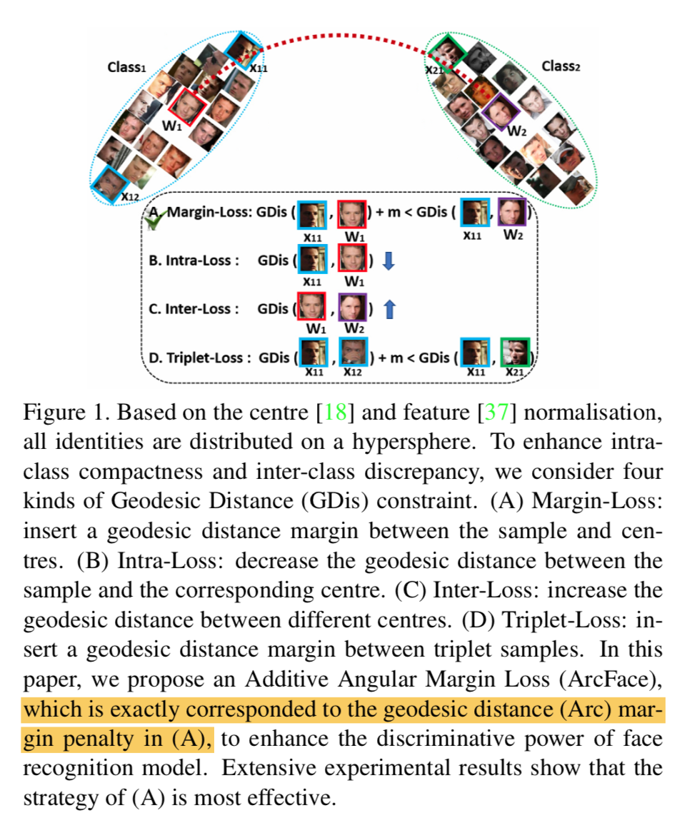
Less is More


  • 首页

  • 标签

  • 归档

  • 搜索

ArcFace

发表于 2022-03-28 |

一些metric loss特点的总结:

* margin-loss:样本与自身类簇心的距离要小于样本与其他类簇心的距离——标准center loss
* intra-loss:对样本和对应类簇心的距离做约束——小于一定距离
* inter-loss:对样本和其他类簇心的距离做约束——大于一定距离
* triplet-loss:样本与同类样本的距离要小于样本与其他类样本的距离

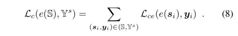
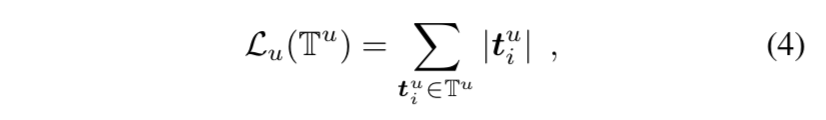
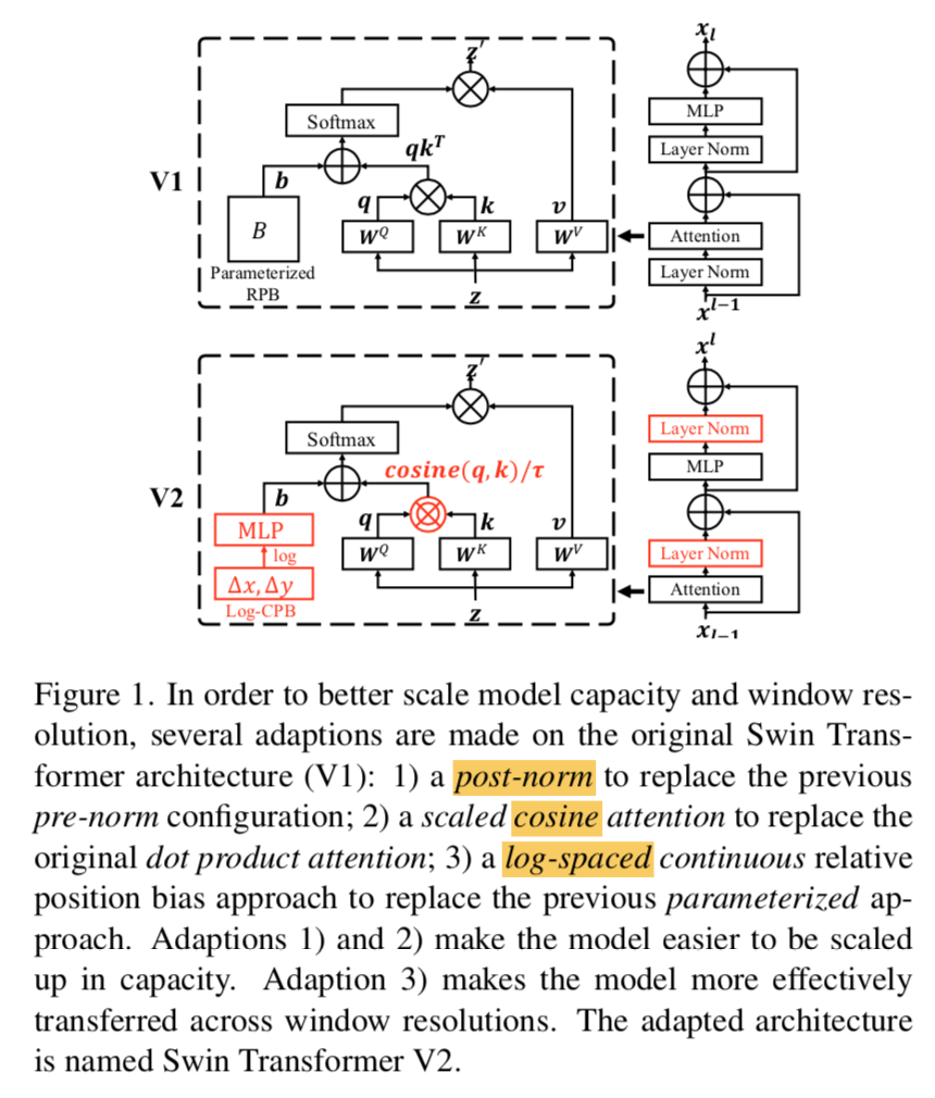
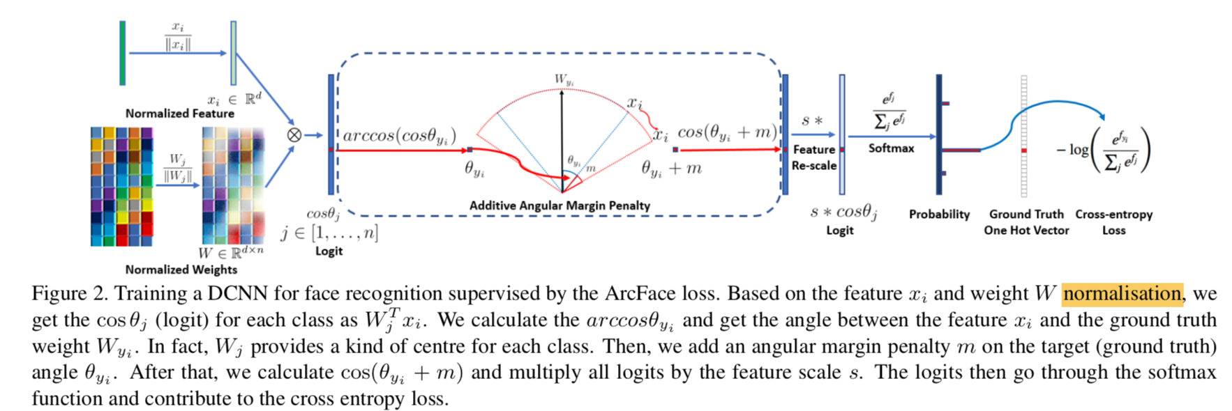
ArcFace: Additive Angular Margin Loss for Deep Face Recognition

  1. 动机

    • 场景:人脸,
    • 常规要素:
      • hypersphere:投影空间
      • metric learning:距离(Angles/Euclidean) & class centres
    • we propose
      • an additive angular margin loss:ArcFace
      • has a clear geometric interpretation
      • SOTA on face & video datasets
  2. 论点

    • face recognition
      • given face image
      • pose normalisation
      • Deep Convolutional Neural Network (DCNN)
      • into feature that has small intra-class and large inter-class distance
    • two main lines
      • train a classifier:softmax
        • 最后的分类层参数量与类别数成正比
        • not discriminative enough for the open-set
      • train embedding:triplet loss
        • triplet-pair的数量激增,大数据集的iterations特别多
        • sampling mining很重要,对精度&收敛速度
    • to enhance softmax loss
      • center loss:在分类的基础上,压缩feature vecs的类内距离
      • multiplicative angular margin penalty:类特别多的时候,center就不好更新了,用last fc weights能够替代center,但是会不稳定
      • CosFace:直接计算logit的cosine margin penalty,better & easier
    • ArcFace
      • improve the discriminative power
      • stabilise the training meanwhile
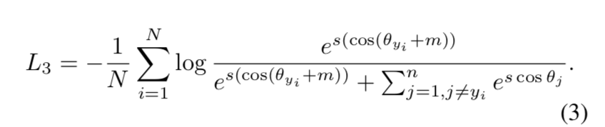
      • margin-loss:Distance(类内)+m < Distance(类间)
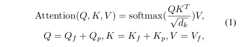
      • 核心idea:normed feature和normed weights的dot product等价于在求他俩的 cosine distance,我们用arccos就能得到feature vec和target weight的夹角,给这个夹角加上一个margin,然后求回cos,作为pred logit,最后softmax
  3. 方法

    • ArcFace

      • transitional softmax

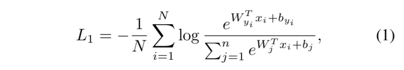
        • not explicitly enforce intra-class similarity & inter-class diversity
        • 对于类内variations大/large-scale测试集的场景往往有performance gap
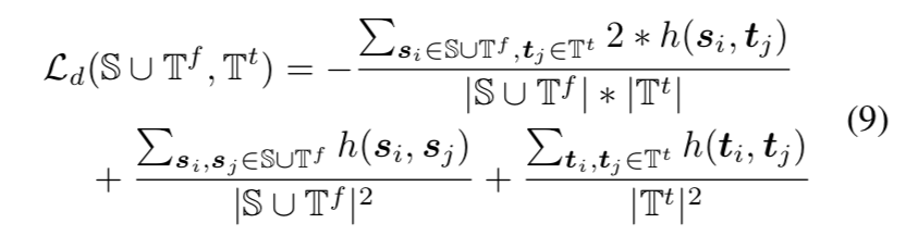
      • our modification

        • fix the bias $b_j=0$ for simplicity

        • transform the logit $W_j^T x=||W_j||\ ||x||cos\theta_j$,$\theta_j$是weight $W_j \in R^d$和样本feature $x \in R^d$的夹角

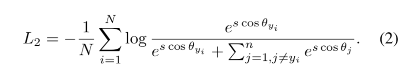
        • fix the $||W_j||$ by l2 norm:$||W_j||=1$

        • fix the embedding $||x||$ by l2 norm and rescale: $||x||=s$

        • thus only depend on angle:这使得feature embedding分布在一个高维球面上,最小化与gt class的轴(对应channel的weight vec,也可以看作class center)夹角

        • add an additive angular margin penalty:simultaneously enhance the intra-class compactness and inter-class discrepancy

        • 作用

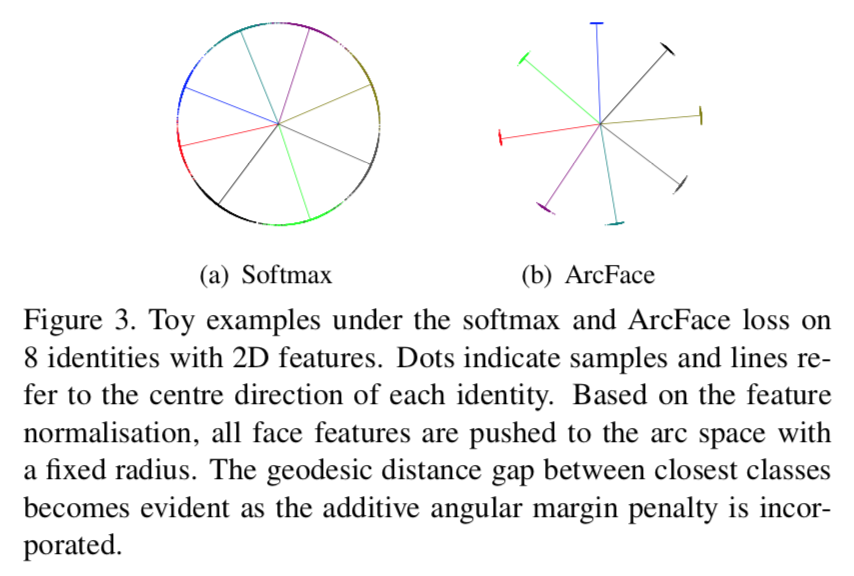
          • softmax produce noticeable ambiguity in decision boundaries
          • ArcFace loss can enforce a more evident gap

      • pipeline

      • 实现

​

DA-WSOL: object localization

发表于 2022-03-21 |

Weakly Supervised Object Localization as Domain Adaption

  1. 动机

    • Weakly supervised object localization (WSOL)
      • localizing objects only with the supervision of image-level classification label
      • previous method use classification structure and CAM to generate the localization score:CAM通常不完全focus在目标上,定位能力weak
    • our method
      • 将任务建模成域迁移任务,domain-adaption(DA) task
      • score estimiator用image-level信息来训练,用像素级信息来测试
      • a DA-WSOL pipeline
        • a target sampling strategy
        • domain adaption localization (DAL) loss
  2. 论点

    • CAM的表现不佳

      • 核心在于domain shift:用分类架构,训练一个分类任务,是对image-level feature的优化,但是目标却是 localization score,这是pixel-level feature,两者之间没有建立联系
      • 最终estimator会get overfitting on source domain(也就是image-level target)
      • 一个直观的想法:引入DA,align the distribution of these two domains,avoid overfitting——activating the discriminative parts of objects
    • mechanisms

      • B: Multi-instance learning(MIL) based WSOL
        • 分类架构
        • 类别目标驱动
        • 通过各种data augmentation/cut mix来strengthen
        • 印象里原论文是先训一个纯分类网络(CNN+fc),然后去掉头,改成CNN+GAP+fc,做finetuning,得到能产生CAM的网络(提取对应类别权重对特征图加权),因为需要两步训练,后面如果要看cam一半都是用grad-cam(用梯度的平均作为权重,无需重新训练),performance据说等价
      • C: Separated-structure based WSOL
        • 一个目标分类任务
        • 一个目标定位任务:伪标签、多阶段
      • A: Domain Adaption
        • 引入DA to better assist WSOL task:align feature distribution between src/tgt domain
        • end-to-end
        • a target sampling strategy
          • target domain features has a much larger scale than source domain features:显然image-level task下,训练出的特征提取器更多的保留前景特征,但是pixel-level下还包含背景之类的
          • sampling旨在选取source-related target samples & source unseen target samples
        • domain adaption localization (DAL) loss
          • 上述的两类samples fed into这个loss
          • source-related target samples:to solve the sample imbal- ance between two domains
          • source unseen target samples:viewed as the Universum to perceive target cues
  3. 方法

    • Revisiting the WOSL

      • task description:给定$image X\in R^{3 \times N} $,3通道N个pixel,需要分辨任意像素$X_{:,i}$是否属于a certain class 0-k
      • a feature extractor f(~):用来提取pixel-level features $Z = f(X) \in R^{C \times N}$
      • a score estimator e(~):用来估计pixel的localization score $Y=e(Z) \in R^{K \times N}$
      • 在有监督场景下,pixel-level target Y是直接给定的,但是在无监督场景下,我们只有image-level mask,即$y=(max(Y_{0:}), max(Y_{1:}), …, max(Y_{k:})) \in R^{K \times 1}$,即每个feature map的global max/avg value构成的feature vector
      • an additional aggregator g (~):用来聚合feature map,将pixel-level feature转换成image-level $z=g(Z) \in R^{C\times 1}$,如GAP
      • 然后再fed into the score estimator above:$y^* = e(z) \in R^{K \times 1}$
      • 用classification loss来监督$y$和$y^*$,这就是一个分类任务
      • but at test time:the estimator is projected back onto the pixel-level feature Z to predict the localization scores,这就是获取CAM
    • Modeling WSOL as Domain Adaption

      • 对每个sample X,建立两个feature sets S & T
        • source domain:$s = z = (gf)(X)$
        • target domain:$\{t_1,t_2,…,t_N\} =\{Z_{1,:},Z{2,:},…,Z{N,:}\}=f(X)$
      • aim at minimizing the target risk without accessing the target label set (pixel-level mask),可以转化为:
        • minimizing source risk
        • minimizing domain discrepancy
        • $L(S,Y^S,T) = L_{cls}(S,Y^S) + L_a(S,T)$
      • loss
        • L_cls就是常规的分类loss,在image-level上train
        • L_a是proposed adaption loss,用来最小化S和T的discrepancy,会force f(~)和g (~)去学习domain-invariant features
        • 使得 e(~)在S和在T上的performance相似
      • properties to notice

        • some samples在set T中存在,而在set S中不存在,如background,不能强行align两个set
        • 两个分布的scale比例十分imbalance,1:N——the S set in some degree insufficient
        • 两个分布的差异是已知的,就是aggregator g (~),这是个先验知识
      • mechanism as in figure

        • 起初两个分布并不一致,方框1/2是image level feature,圆圈1/2是pixel level feature,圆圈问号类是pixel map上的bg patches
        • 用class loss去监督如CAM method,能够区分方框1/2,在一定程度上也能够区分圆圈1/2,但是不能精准定位目标,因为S和T存在discrepancy——bg patches
        • 引入domain adaption loss,能够tighten两个set,使得两个分布更加align,这样class bound在方框1/2和圆圈1/2上的效果都一样好
        • 引入Universum regularization,推动decision boundary into Universum samples,使得分类边界也有意义

    • Domain Adaption Localization Loss $L_a$(~)

      • 首先进一步切分target set T
        • Universum $T^u$:不包含前景类别/bg样本
        • the fake $T^f$:和source domain的sample highly correlated的样本(在GAP时候被保留下来的样本)
        • the real $T^t$:aside from above two的样本
      • recall the properties
        • the fake之所以会highly correlated source domain,就是因为先验知识GAP (property3),我们知道他就是在GAP阶段被留下来的target sample
        • 我们可以将其作为source domain的补充样本,以弥补insufficient issue (property2)
        • 关于unmatched data space (property1),T-Universum就与S保持same label space了
      • based on these subsets,overall的DAL loss包含两个部分
        • domain adaption loss $L_d$:UDA,unsupervised,align the distribution
        • Universum regularization $L_u$:feature-based L1 regularization,所有bg像素的绝对值之和,如果他们都在分类边界上,不属于任何一个前景类,localization score的响应值就都是0,那么loss就是0
        • $L_a(S,T) = \lambda_1L_d(S \cup T^f, T^t) + \lambda_2 L_u(T^u)$
    • Target Sampling Strategy (这个有点不太理解)

      • a target sample assigner(TSA)
      • a cache matrix $M \in R^{C \times (K+1)}$
        • column 0:represents the anchor of $T^u$
        • the rest column:represents the anchor of certain class of $T^t$
        • 感觉就是记录了每类column vec的簇心
      • init

        • column 0:zero-init
        • the rest:当遇到第一个这一类的样本的时候,用src vec $z+\epsilon$初始化
      • update

        • 首先基于image-level label得到类别id:$k = argmax(y)$,注意使用ground truth,不是prediction vec
        • 然后拿到cache matrix中对应的anchor:$a^u = M_{:,0}, \ \ a^t = M_{:,k+1}$
        • 然后再加上image-level predict作为初始的cluster:$C_{init} = \{a^u, a^t, z\} \in R^{C \times 3}$
        • 对当前target samples做K-means,得到三类样本,进而计算adaption loss
        • 用聚类得到的新center C,加权平均更新cache matrix,权重$r_k$是对应类images的数目的倒数

      • overall

    • pipeline summary

      • 首先获得S和T,f(~)是classification backbone(resnet/inception),g(~)是 global average pooling,e(~)是作用在source domain feature vector的 fully-connected layer ,generate the image-level classification score,supervised with cross-entropy

      • 然后通过S、T以及ground truth label id得到3个target subsets

        • $T^u$用来计算$L_u$

        • $S$和$T^f$和$T^t$用来计算$L_d$:MMD (Maximum Mean Discrepancy),h(~)是高斯kernel

ImageSearch

发表于 2022-03-07 |

以图搜图

  1. 两大类

    • pHash + hamming距离
    • CNN + cos距离
  2. pHash

    cv2的dct变换和库函数imagehash调用的scipy.fftpack.dct结果不太一样,所以编码结果也不一样

    1
    2
    3
    4
    5
    6
    7
    8
    9
    10
    11
    12
    13
    14
    15
    16
    17
    18
    19
    20
    21
    22
    23
    24
    25
    26
    27
    import numpy as np
    import cv2
    import imagehash
    from PIL import Image


    def pHash(img_file):

    # step1: gray, 0-255, 32x32
    img = cv2.imread(img_file, 0)
    img = cv2.resize(img, (32,32), interpolation=cv2.INTER_CUBIC)

    # step2: dct, left-top 8x8
    img = cv2.dct(img.astype(np.float32))
    img = img[:8,:8]

    # step3: flatten, mean, 0-1 binary
    img = img.reshape((-1)).tolist()
    mean = sum(img)/len(img)
    img_print = ['1' if i>mean else '0' for i in img]

    # hex encoding
    return ''.join(['%x' % int(''.join(img_print[i:i+4]),2) for i in range(0,32*32,4)])

    cv_hash = pHash(img_file)
    scipy_hash = imagehash.phash(Image.open(img_file), hash_size=8, highfreq_factor=4) # imagehash object
    scipy_hash = scipy_hash.__str__()

    以上编码得到16位的16进制编码,类似这张图像的低级特征指纹。

    Hamming距离:两个等长字符串,在对应位置的不同字符的个数

    • 如果不同字符数不超过5,说明近似
    • 如果大于10,说明不同

Faiss

发表于 2022-03-02 |

Faiss: A library for efficient similarity search

  1. official site:

    主页:https://ai.facebook.com/tools/faiss/

    repo/wiki:https://github.com/facebookresearch/faiss

HMC: Hierarchical Multi-Label Classification Networks

发表于 2022-02-25 |

ICML2018,multi-label,hierarchical

理想数据集的类别间是互斥的,但是现实往往存在层级/包含关系,多个数据集合并时也会有这个情况

reference code: https://github.com/Tencent/NeuralNLP-NeuralClassifier/blob/master/model/classification/hmcn.py

HMCN: Hierarchical Multi-Label Classification Networks

  1. 动机

    • HMC:hierarchical multi-label classification
      • classes are hierarchically structured,类别是有层级关系的
      • objects can be assigned to multiple paths,目标可能点亮多条tree path——多标签
    • application domains
      • text classification
      • image annotation
      • bioinformatics tasks such as protein function prediction
    • propose HMCN
      • local + global loss
      • local:discover local hierarchical class-relationships
      • global:global information from the entire class while penalizing hierarchical violations
  2. 论点

    • common methods
      • local-based:
        • 建立层级的top-down局部分类器,每个局部分类器用于区分当前层级,combine losses
        • computation expensive,更善于提取wordTree局部的信息,容易overfitting
      • global-based:
        • 只有一个分类器,将global structure associate起来
        • cheap,没有error-propagation problem,容易underfitting
    • our novel approach
      • combine两者的优点
      • recurrent / non-recurrent版本都有
      • 由multiple outputs构成
        • 每个class hierarchy level有一个输出:local output
        • 全局还有一个global output
      • also introduce a hierarchical violation penalty
  3. 方法

    • a feed-forward architecture (HMCN-F)

      • notations
        • feature vec $x \in R^{D}$:输入向量
        • $C^h$:每层的节点
        • $|H|$:总层数
        • $|C|$:总类数
      • global flow
        • 第一行横向的data flow
        • 将$i^{th}$层的信息carry到第$(i+1)^{th}$层
        • 第一层:$A_G^1 = \phi(W_G^1 x +b_G^1)$
        • 接下来的层:$A_G^h = \phi(W_G^h(A_G^{h-1} \odot x) +b_G^h)$
        • 最终的global prediction:$P_G=\sigma(W_G^{H+1}A_G^{H}+b_G^{H+1}) \in R^{|C|}$
      • local flow
        • start from 每个level的global hidden layer
        • local hidden layer:$A_L^h = \phi(W_T^hA_G^{h} +b_T^h)$
        • local prediction:$P_L^h = \sigma(W_L^hA_L^{h} +b_L^h) \in R^{C^h}$
      • merge information
        • 将local的prediction vectors concat起来
        • 然后和global preds相加
        • $P_F = \beta (P_L^1 \odot P_L^2 \odot… P_L^1) + (1-\beta) P_G$
      • hyperparams
        • $\beta=0.5$
        • fc-bn-dropout:dim=384,drop_rate=0.6
    • a recurrent architecture (HMCN-R)

    • training details

      • small datasets with large number of classes
      • Adam
      • lr=1e-3
  4. 实验

    • 【小batch反而结果更好】one can achieve better results by training HMCN models with smaller batches

YOLO9000: 回顾yolov2的wordTree

  1. 动机

    • 联合训练,为了扩展类数
      • 检测样本梯度回传full loss
      • 分类样本只梯度回传分类loss
  2. Hierarchical classification

    • 构建WordTree

    • 对每个节点的预测是一个条件概率:$Pr(child_node|parent_node)$

    • 这个节点的绝对概率是整条链路的乘积

    • 每个样本的根节点概率$Pr(object)$是1

    • 对每个节点下面的所有children做softmax

    • 首先论文就先用darknet19训了一个1369个节点的层次分类任务

      • 1000类flat softmax on ImageNet:72.9% top-1,91.2% top-5
      • 1369类wordTree softmax on ImageNet:71.9% top-1,90.4% top-5
      • 观察到Performance degrades gracefully:总体精度下降很少,而且即使分不清是什么狗品种,狗这一类的概率还是能比较高
    • 然后用在检测上

      • 每个目标框的根节点概率$Pr(object)$是yolo的obj prob
      • 仍旧对每个节点做softmax,标签是高于0.5的最深节点,不用连乘条件概率
        • take the highest confidence path at every split
        • until we reach some threshold
        • and we predict that object class
      • 对一个分类样本
        • 我们用全图类别概率最大的bounding box,作为它的分类概率
        • 然后还有objectness loss,预测的obj prob用0.3IOU来threshold:即如果这个bnd box的obj prob<0.3是要算漏检的

ConvNext

发表于 2022-01-21 |

facebook,2022,https://github.com/facebookresearch/ConvNeXt

inductive biases(归纳偏置)

  • 卷积具有较强的归纳偏置:即strong man-made settings,如local kernel和shared weights,只有spatial neighbor之间有关联,且在不同位置提取特征的卷积核共享——视觉边角特征与空间位置无关
  • 相比之下,transformer结构就没有这种很人为的先验的设定,就是global的优化目标,所以收敛也慢

A ConvNet for the 2020s

  1. 动机

    • reexamine the design spaces and test the limits of what a pure ConvNet can achieve
    • 精度
      • achieving 87.8% ImageNet top-1 acc
      • outperforming Swin Transformers on COCO detection and ADE20K segmentation
  2. 论点

    • conv
      • a sliding window strategy is intrinsic
      • built-in inductive biases:卷积的归纳偏置是locality和spatial invariance
        • 即空间相近的grid elements有联系而远的没有:translation equivariance is a desirable property
        • 空间不变性:shared weights,inherently efficient
    • ViT
      • 除了第一层的patchify layer引入卷积,其余结构introduces no image-specific inductive bias
      • global attention这个设定的主要问题是平方型增长的计算量
      • 使得这个结构在classification任务上比较work,但是在其他任务场景里面(需要high resolution,需要hierarchical features)使用受限
    • Hierarchical Transformers
      • hybrid approach:重新引入local attention这个理念
      • 能够用于各类任务
      • 揭露了卷积/locality的重要性
    • this paper brings back convolutions
      • propose a family of pure ConvNets called ConvNeXt
      • a Roadmap:from ResNet to ConvNet
  3. 方法

    • from ResNet to ConvNet

      • ResNet-50 / Swin-T:FLOPs around 4.5e9
      • ResNet-200 / Swin-B around 15e9
      • 首先用transformer的训练技巧训练初始的resnet,作为baseline,然后逐步改进结构

        • macro design
        • ResNeXt
        • inverted bottleneck
        • large kernel size
        • various layer-wise micro designs

    • Training Techniques

      • 300 epochs
      • AdamW
      • aug:Mixup,CutMix,RandAugment,Random Erasing
      • reg:Stochastic Depth,Label Smoothing
      • 这就使得resnet的精度从76.1%提升到78.8%

    • Macro Design

      • 宏观结构就是multi-stage,每个stage的resolution不同,涉及的结构设计有
        • stage compute ratio
        • stem cell
      • swin的stage比是1:1:3:1,larger model是1:1:9:1,因此将resnet50的3:4:6:3调整成3:3:9:3,acc从 78.8% 提升至 79.4%
      • 将stem替换成更加aggressive的patchify,4x4conv,s4,non-overlapping,acc从 79.4% 提升至 79.5%
    • ResNeXt-ify

      • 用分组卷积来实现更好的FLOPs/acc的trade-off
      • 分组卷积带来的model capacity loss用增加网络宽度来实现
      • 使用depthwise convolution,同时width从64提升到96
        • groups=channels
        • similar to the weighted sum of self-attention:在spatial-dim上mix information
      • acc提升至80.5%,FLOPs增加5.3G
    • Inverted Bottleneck

      • transformer block的ffn中,hidden layer的宽度是输入宽度的4倍

      • MobileNet & EfficientNet里面也有类似的结构:中间大,头尾小

      • 而原始的resne(X)t是bottleneck结构:中间小,两头大,为了节约计算量

      • reduce FLOPs:因为shortcut上面的1x1计算量小了
      • 精度稍有提升:80.5% to 80.6%,R200/Swin-B上则更显著一点,81.9% to 82.6%
    • Large Kernel Sizes

      • 首先将conv layer提前,类比transformer的MSA+FFN
      • reduce FLOPs,同时精度下降至79.9%
      • 然后增大kernel size,尝试[3,5,7,9,11],发现在7的时候精度饱和
      • acc:from 79.9% (3×3) to 80.6% (7×7)
    • Micro Design:layer-level的一些尝试

      • Replacing ReLU with GELU:原始的transformer paper里面也是用的ReLU,但是后面的先进transformer里面大量用了GeLU,实验发现可以替换,但是精度不变
      • Fewer activation functions:transformer block里面有QKV dense,有proj dense,还有FFN里的两个fc层,其中只有FFN的hidden layer接了个GeLU,而原始的resnet每个conv后面都加了relu,我们将resnet也改成只有类似线性层的两个1x1 conv之间有激活函数,acc提升至81.3%,nearly match Swin
      • Fewer normalization layers:我们比transformer还少用一个norm(因为实验发现加上入口那个LN没提升),acc提升至81.4%,already surpass Swin

      • Substituting BN with LN:BN对于convNet,能够加快收敛抑制过拟合,直接给resnet替换LN会导致精度下降,但是在逐步改进的block上面替换则会slightly提升,81.5%

      • Separate downsampling layers:学Swin,不再将stride2嵌入resnet conv,而是使用独立的2x2 s2conv,同时发现在resolution改变的时候加入norm layer能够stabilize training——每个downsamp layer/stem/final GAP之后都加一个LN,acc提升至82%,significantly exceeding Swin

    • overall structural params

how to train ViT

发表于 2022-01-20 |

炼丹大法:

[Google 2021] How to train your ViT? Data, Augmentation, and Regularization in Vision Transformers,Google,rwightman,这些个点其实原论文都提到过了,相当于补充实验了

[Google 2022] Model soups: averaging weights of multiple fine-tuned models improves accuracy without increasing inference time,多个模型权重做平均

[Facebook DeiT 2021] Training data-efficient image transformers & distillation through attention,常规技巧大全

How to train your ViT? Data, Augmentation, and Regularization in Vision Transformers

  1. 动机

    • ViT vs. CNN
      • 没有了平移不变形
      • requires large dataset and strong AugReg
    • 这篇paper的contribution是用大量实验说明,carefully selected regularization and augmentation比憨憨增加10倍数据量有用,简单讲就是在超参方面给一些insight
  2. 方法

    • basic setup

      • pre-training + transfer-learning:是在google research的原版代码上,TPU上跑的

      • inference是在timm的torch ViT,用V100跑的

      • data

        • pretraining:imagenet
        • transfer:cifar
      • models

        • [ViT-Ti, ViT-S, ViT-B and ViT-L][https://github.com/rwightman/pytorch-image-models/blob/master/timm/models/vision_transformer.py]
        • 决定模型scale的几个要素:
          • depth:12,24,32,40,48
          • embed_dim:192,384,768,1024,1280,1408
          • mlp_ratio:4,48/11,64/13
          • num_heads:3,6,12,16
        • 还有影响计算量的变量:
          • resolution:224,384
          • patch_size:8,16,32
        • 和原版唯一的不同点是去掉了MLP head里面的hidden layer——那个fc-tanh,据说没有performance提升,还会引发optimization instabilities

    • Regularization and data augmentations

      • dropout after each dense-act except the Dense_QKV:0.1
      • stochastic depth:线性增长dbr,till 0.1
      • Mixup:beta分布的alpha
      • RandAugment:randLayers L & randMagnitude M
      • weight decay:0.1 / 0.03,注意这个weight decay是裸的,实际计算是new_p = new_p - p*weight_decay*lr,这个WD*lr可以看作实际的weight decay,也就1e-4/-5量级
    • Pre-training

      • Adam:[0.9,0.999]
      • batch size:4096
      • cosine lr schedule with linear warmup(10k steps)
      • gradients clip at global norm 1
      • crop & random horizontal flipping
      • epochs:ImageNet-1k 300 epochs,ImageNet-21k [30,300] epochs
    • Fine-tuning

      • SGD:0.9
      • batch size:512
      • cosine lr schedule with linear warmup
      • gradients clip at global norm 1
      • resolution:[224,384]
  3. 结论

    • Scaling datasets with AugReg and compute:加大数据量,加强aug&reg

      • proper的AugReg和10x的数据量都能引导模型精度提升,而且是差不多的水平

    • Transfer is the better option:永远用预权重去transfer,尤其大模型

      • 在数据量有限的情况下,train from scratch基本上不能追上transfer learning的精度

    • More data yields more generic models:加大数据,越大范化性越好

    • Prefer augmentation to regularization:非要比的话aug > reg,成年人两个都要

      • for mid-size dataset like ImageNet-1k any kind of AugReg helps
      • for a larger dataset like ImageNet-21k regularization almost hurts,但是aug始终有用

    • Choosing which pre-trained model to transfer

    • Prefer increasing patch-size to shrinking model-size:显存有限情况下优先加大patch size
      • 相似的计算时间,Ti-16要比S-32差
      • 因为patch-size只影响计算量,而model-size影响了参数量,直接影响模型性能

Training data-efficient image transformers & distillation through attention

  1. 动机

    • 大数据+大模型的高精度模型不是谁都负担得起的
    • we produce competitive model
      • use Imagenet only
      • on single computer,8-gpu
      • less than 3 days,53 hours pretraining + 20 hours finetuning
      • 模型:86M,top-1 83.1%
      • 脸厂接地气!!!
    • we also propose a tranformer-specific teacher-student strategy
      • token-based distillation
      • use a convnet as teacher
  2. 论点

    • 本文就是在探索训练transformer的hyper-parameters、各种训练技巧

    • Knowledge Distillation (KD)

      • 本文主要关注teacher-student
      • 用teacher生成的softmax结果(soft label)去训练学生,相当于用student蒸馏teacher
    • the class token
      • a trainable vector
      • 和patch token接在一起
      • 然后接transformer layers
      • 然后 projected with a linear layer to predict the class
      • 这种结构force self-attention在patch token和class token之间进行信息交换
      • 因为class token是唯一的监督信息,而patch token是唯一的输入变量
    • contributions
      • scaling down models:DeiT-S和DeiT-Ti,向下挑战resnet50和resnet18
      • introduce a new distillation procedure based on a distillation token,类似class token的角色
      • 特殊的distillation机制使得transformer相比较于从同类结构更能从convnet上学到更多
      • well transfer
  3. 方法

    • 首先假设我们有了一个strong teacher,我们的任务是通过exploiting the teacher来训练一个高质量的transformer

    • Soft distillation

      • teacher的softmax logits不直接做标签,而是计算两个KL divergence
      • CE + KL loss

    • Hard-label distillation

      • 就直接用作label
      • CE + CE

      • 实验发现hard比soft结果好

    • Distillation token

      • 在token list上再添加一个new token
      • 跟class token的工作任务一样
      • distillation token的优化目标是上述loss的distillation component
      • 与class token相辅相成
      • 作为对比,也尝试了用原本的CE loss训练两个独立的class token,发现这样最终两个class token的cosine similarity高度接近1,说明额外的class token没有带来有用的东西,但是class token和distillation token的相似度最多也就0.93,说明distillation branch给模型add something,【难道不是因为target不同所以才不同吗???】

    • Fine-tuning with distillation

      • finetuning阶段用teacher label还是ground truth label?
      • 实验结果是teacher label好一点
    • Joint classifiers

      • 两个softmax head相加
      • 然后make the prediction
  4. Training details & ablation

    • Initialization

      • Transformers are highly sensitive to initialization,可能会导致不收敛
      • 推荐是weights用truncated normal distribution
    • Data-Augmentation

      • Auto-Augment, Rand-Augment, random erasing, Mixup等等
      • transformers require a strong data augmentation:几乎都有用
      • 除了Dropout:所以我们把Dropout置零了

    • Optimizers & Regularization

      • AdamW
      • 和ViT一样的learning rate
      • 但是much smaller weight decay:发现weight decay会hurt convergence

MAE

发表于 2022-01-13 |

papers

[MAE] Masked Autoencoders Are Scalable Vision Learners:恺明,将BERT的掩码自监督模式搬到图像领域,设计基于masked patches的图像重建任务

[VideoMAE] VideoMAE: Masked Autoencoders are Data-Efficient Learners for Self-Supervised Video Pre-Training:腾讯AI Lab,进一步搬运到video领域

Masked Autoencoders Are Scalable Vision Learners

  1. 动机

    • 一种自监督训练(pretraining)方式,用来提升模型泛化性能
    • 技术方案:
      • mask & reconstruct
      • encoder-decoder architecture
        • encoder operates only on visible patches:首先对input patches做random sampling,只选取少量patches给到encoder
        • lightweight decoder run reconstruction on (masked) tokens:将encoded patches和mask tokens组合,给到decoder,用于重建原始图像
    • 精度
      • with MAE pretraining,ViT-Huge on ImageNet-1k:87.8%
  2. 论点

    • 自监督路线能给到模型更大体量的数据,like NLP,masked autoencoding也是经典的BERT训练方式,but现实是autoencoding methods in vision lags behind NLP

      • information density:NLP是通过提取高级语义信息去推断空缺的,而图像如果有充足的邻里低级空间信息,就能重建出来不错的效果,导致模型没学到啥高级语义信息就收敛了,本文的解决方案是random mask极大比例的patches,largely reduce redundancy
      • decoder plays a different role be- tween reconstructing text and images:和上一条呼应,visual decoder重建的是像素,低级信息,NLP decoder重建的是词向量,是高级表征,因此BERT用了个贼微小的结构来建模decoder——一个MLP,但是图像这边decoder的设计就重要的多——plays a key role in determining the semantic level of the learned latent representations
    • our MAE

      • 不对称encoder-decoder
      • high portion masking:既提升acc又减少计算量,easy to scale-up
      • workflow

        • MAE pretraing:encode random sampled patches,decode encoded&masked tokens
        • down stream task:save encoder for recognition tasks

  3. 方法

    • masking
      • 切分图像:non-overlapping patches
      • 随机采样:random sample the patches following a uniform distribution
      • high masking ratio:一定要构建这样的task,不能简单通过邻里低级信息恢复出来,必须要深入挖掘高级语义信息,才能推断出空缺是啥
    • MAE encoder
      • ViT
      • given patches:linear proj + PE
      • operates on a small visible subset(25%) of the full set
      • 负责recognition任务
    • MAE decoder
      • a series of Transformer blocks:远小于encoder,narrower and shallower,单个token的计算量是encoder的<10%
      • given full set tokens
        • mask tokens:a shared & learned vector 用来表征missing patches
        • add PE:从而区别不同的mask token
      • 负责reconstruction任务
    • Reconstruction target
      • decoder gives the full set reconstructed tokens:[b,N,D]
        • N:patch sequence length
        • D:patch pixel values
      • reshape:[b,H,W,C]
      • 重建loss,per-pixel MSE:compute only on masked patches
      • 【QUESTION,这个还没理解】还有一个变体,官方代码里叫norm_pix_loss,声称是for better representation learning,以每个patch的norm作为target:
        • 对每个masked patch,计算mean&std,
        • 然后normalize,
        • 这个normed patch作为reconstruction target

det-transformers

发表于 2021-12-08 |
  • 目标检测leaderboard: https://paperswithcode.com/sota/object-detection-on-coco
    • boxAP
    • swin开启了霸榜时代:家族第一名63.1
    • 接着是YOLO家族:家族第一名57.3,YOLOv4是55.8
    • DETR:论文里是44.9(没在榜单上),只有一个deformable DETR是52.3
    • 时代的眼泪Cascade Mask R-CNN:42.8
    • anchor-free系列:FCOS是44.7,centerNet是43.5
  • 目前检测架构的几个霸榜算法
    • DETR系列end-to-end
    • Swin放在传统二阶段架构里面
    • YOLO
    • tricks加持:multi-scale、TTA、self-training、cascade、GIoU
  • papers

    [DETR 2020] End-to-End Object Detection with Transformers:Facebook,首个端到端检测架构,无需nms等后处理,难优化,MSA的显存/计算量

    [Swin 2021] Swin Transformer: Hierarchical Vision Transformer using Shifted Windows:微软,主要是swin-back的建模能力强,放在啥框架里都很行

    [deformable DETR 2021] DEFORMABLE DETR: DEFORMABLE TRANSFORMERS FOR END-TO-END OBJECT DETECTION:商汤,将MSA卷积话,解决transformer的high-resolution困境

    [anchor DETR 2022] Anchor DETR: Query Design for Transformer-Based Object Detection:旷视,new query design,也是针对attention结构的变种(cross-attention),精度更高,显存更少,速度更快,收敛更快

    [DDQ 2022] What Are Expected Queries in End-to-End Object Detection? 商汤,基于DETR,讨论新的dense queries

  • repo

    https://github.com/facebookresearch/detr

    https://github.com/facebookresearch/3detr,3D版本

    https://github.com/fundamentalvision/Deformable-DETR

    https://github.com/megvii-research/AnchorDETR

    https://github.com/jshilong/DDQ,暂时没开源代码,只有主页

Swin details for object detection

  1. integrate Swin backbone into 4 frameworks in mmdetection

    • Cascade Mask R-CNN
    • ATSS
    • RepPoints v2
    • Sparse RCNN
  2. basic setttings

    • multi-scale training:resize输入使得shorter side is between 480 and 800
    • AdamW:lr=0.0001,weight decay=0.05
    • batch size=16
    • stochastic depth=0.2
    • 3x schedule (36 epochs with the learn- ing rate decayed by 10× at epochs 27 and 33)
    • pretrained:use a ImageNet-22K pre-trained model as initialization
  3. compare to ResNe(X)t

    • R50 vs. Swin-T:Swin-T普遍优于R50,4个框架Cascade Mask R-CNN > RepPoints V2 > Sparse R-CNN > ATSS

    • X101 vs. Swin-S & X101-64 vs. Swin-B:Swin普遍优于RX

    • System-level Comparison:进一步加强Swin-L

      • HTC++
      • stonger multi-scale input(400-1400)
      • 6x schedule (72 epochs)
      • soft- NMS
      • ImageNet-22K pre-trained

DETR: End-to-End Object Detection with Transformers

第一次看时有些技术细节不太理解,重新梳理一下:

  1. encoder

    • feature inputs:
      • 用了resnet最后一个阶段的输出,(H0/32,W0/32,C),C=2048
      • 然后用1x1 conv降维,(H,W,d),作为attention layer的输入
    • 没有batch dim,one image per GPU,外加DDP
    • DC:distillation conv
    • fixed PE:
      • 给每一层attention layer的输入query和key都加了fixed PE
      • 注意是QK不是QKV
      • 论文的示例代码为了简洁用了learnt PE,而且只加在input层
  2. decoder

    • object queries:全0初始化,100是建议长度,补充材料里面有个实验,图像包含40以下目标时候基本不会漏检,再往上就开始漏检了
    • learnt PE
  3. prediction heads

    • 首先做bipartite matching

      • 将pred box和gt box一一对应,没配上的pred box与no object对齐

      • matching loss:寻找到最优的pred box排列,使得matching cost最小,优化算法是Hungarian algorithm,matching cost也可以理解为匹配质量

        • 第一项是匹配上的某个box,它的预测概率,越大说明越confident,匹配质量越好

        • 第二项是匹配上的某个box,它与gtbox的box loss,越大匹配质量越不好

    • 然后计算detection loss

      • cls loss:CE
      • box loss:L1 + GIoU

DEFORMABLE DETR: DEFORMABLE TRANSFORMERS FOR END-TO-END OBJECT DETECTION

  1. 动机

    • DETR的痛点
      • slow convergence
      • limited feature spatial resolution:小目标往往需要放大输入resolution才能检出,但是transformer负担不起high-resolution计算
    • 处理attention module的计算限制
      • only attend to a small set of key sampling points
      • 那应该类似两阶段?先选格子,再fine-regress
    • performace
      • better than DETR
      • 10x less training epochs
      • 两阶段架构上,用作RPN,performance有进一步提升
  2. 论点

    • Modern object detectors:not fully end-to-end

      • anchor
      • training target assignment
      • NMS

      • 都是hand-crafted components,引入了超参的

    • DETR:fully end-to-end

      • 直接回归box,结构极简
      • 但是有痛点
        • high-resolution
        • slow convergence:attention weights需要很久才能focus到sparse object上
    • deformable convolution

      • a powerful and efficient mech- anism to attend to sparse spatial locations
      • while lacks the element relation modeling mechanism
    • we propose Deformable DETR

      • combines the best of deformable conv and Transformers

        • deformable conv:sparse spatial sampling
        • Transformers:relation modeling capability
      • deformable attention module

        • 替换原始的Transformer attention modules
        • 不是在all featuremap pixels上做计算,而是先pre-filter一部分locations
        • 可以extended to multi-scale:naturally aggregate,无需特征金字塔

  3. 核心技术回顾

    • Multi-Head Attention in Transformers

      • given Q,K,V
      • attention values:$Softmax(\frac{QK^T}{\sqrt d}) V$
      • multi-head:concat + dense
      • 计算量随着feature map的size的二次方增长
    • DETR

      • given CNN feature maps
      • 用一个encoer-decoder的结构,将feature maps转化成a set of object queries
      • encoder是self-attention:Q和K都是feature map pixels
      • decoder是cross-attention + self-attention:

        • cross的query来自decoder的额外输入——N object queries represented by learnable positional embeddings,key来自encoder
        • self的query和key都是decoder的额外输入——object queries

  4. 方法

    • Deformable Attention Module

      • Transformer的attention layer的计算量和feature map的size正相关

      • Deformable attention的一个点,只和周围一个固定pattern上的点计算relationship,控制了计算量

      • assign only a small fixed number of keys for each query

      • 公式

        • given:input $x\in R^{C\times H\times W}$,2d point $p_q$,query feature $z_q$
        • $m$ indexes the attention head
        • $k$ indexes the sampled keys
        • $K$ is the total sampled key number:远小于HW
        • $A_{mqk}$和$\Delta p_{mqk}$是每个head的attention weights & sampling offsets,是从输入feature经过一个线性层得到的
          • 前者还加了一个softmax,normed into [0,1]
          • 后者是feature level的绝对距离,范围无界
        • $W_m^{‘}x_q$是query values
        • $x(p_q + \Delta_p{mqk})$用了bilinear interpolation
    • Multi-scale Deformable Attention Module

      • 将坐标$p_q$转换成normalized形式$\hat p_q$,输入一组不同scale的inputs feature map,将不同scale上这个点的weighted query加在一起就好了

      • 公式

        • $A_{mlqk}$ is normalized by $\sum_{l=1}^L \sum_{k=1}^K A_{mlqk}=1$:attention weights的softmax是在所有level feature的sampled points上的,也就是LK个points
        • $\phi(\hat p_q)$将normed coords转换到对应feature level

    • Deformable Transformer Encoder

      • C3-C6,L=4,channel=256

        • 用Resnet stage3到stage5的featuremap接一个1x1conv,作为multi-scale feature maps
        • C5的output再接一下3x3 s2 conv得到C6

      • 堆叠Multi-scale Deformable Attention Module

        • module的输入和输出都是same resolution的feature maps
        • add a scale-level embedding $e_l$:用来指示输入的query pixel来自哪个scale level,但是它是随机初始化的,然后随着网络训练【???】
        • query是pixels,reference points就是它自身:代码里是query embed + fc来实现
    • Deformable Transformer Decoder

      • cross-attention
        • query是object queries
        • key是encoder的输出
        • object queries are extracting features from the feature maps
      • self-attention
        • query和key都是object queries
        • object queries interact with each other
      • 这里仅给cross-attention module用了Multi-scale Deformable Attention Module,因为decoder的self-att的key不是feature maps了
    • query的reference points is predicted from its object query embedding:fc + sigmoid,也作为box center的initial guess

    • detection head预测的是reference point的偏移量

Anchor DETR: Query Design for Transformer-Based Object Detection

  1. 动机

    • previous DETRs
      • decoder输入的object queries是一系列learned embeddings
      • do not have explicit physical meanings
      • difficult to optimize
    • we propose Anchor DETR
      • a novel query design based on anchors:enable ‘one region multiple objects’
      • an attention variant:reduce memory
      • better performance and fewer training epochs
    • verified on
      • MSCOCO
      • ResNet50-DC5 feature,44.2 AP with 19 FPS
  2. 论点

    • Visualization of the prediction slots

      • a图是DETR的prediction boxes的中心点,绿-红-蓝表示box由小到大,可以看到绿box分布在全图,红蓝则集中在中心,其实类似枚举,没有什么物理意义

      • b图是Anchor DETR的prediction slots,黑点是anchor points,可以看到box的中心点都分布在anchor附近

      • 说明本文方法are more related to a specific position than DETR

    • 回看CNN

      • anchors are highly related to position
      • contain interpretable physical meanings
    • we propose this novel query design

      • 首先用anchor coordinates去编码query
      • 其次针对一个位置多个目标的情况:adding multiple patterns to each anchor point
      • CNN是highly anchor-driven,位置和尺寸都包含了,DETR是完全放飞,随意初始化,本文方法在中间,用了anchor position,但是没有scale
      • 这样还是保证网络预测的格子都在anchor附近:easier to optimize
    • we also propose an attention variant that we call Row-Column Decouple Attention (RCDA)

      • 行列解耦:2D key feature decouple into 1D row and 1D column
      • 串行执行row attention & column attention
      • reduce memory cost

      • similar or better performance

      • 这个其实可以理解的,MSA的global attention太dense computation了,所以才会出现Swin那种WMSA去分块,deformable DETR那种先filter出attention区域,包括本文的解耦,都是在尝试稀疏化
  3. 方法

    • anchor points

      • CNN detector里面anchor points永远对应着feature grids

      • 但是在transformer里面,这个点可以更flexible,可以是learned points sequence

      • 本文两种都尝试了

        • fixed anchor points就是grid coordinates
        • learned anchors就是random uniform初始化,然后加入learned layers,最后输出的learned coordinates

      • 最终的网络预测都加在这个anchor coordinates上,也就是网络又变成预测偏移量了

    • attention formulation:the DETR-like attention

      • 也就是最原始的transformer里面的MSA,QKV首先各自过一层linear layer,然后如下计算:

      • 下标f是feature,下标p是position

      • decoder里面有两种attention:self-attention和cross-attention
        • self-attention里面$Q_f,K_f, V_f$是一样的,来自前面的输出,$Q_p, K_p$是一样的,来自learned positional embedding
        • decoder的第一个query输入$Q^{init}_f \in R^{N_q \times D}$可以是一个常量/一个learned embedding
        • cross-attention里面Q的来源不变,但是KV变成了encoder的输出,$K_p$是sine-cosine positional embedding,是个常量
    • anchor points to object query

      • 原始的DETR用learned positional embedding作为object query,用来distinguishing different objects,缺少可解释性
      • we use anchor points $Pos_q \in R^{N_A \times 2}$
        • $N_A$个点坐标
        • 2是xy-dim,range 0-1
      • encode as the object queries $Q_p$
        • we use a small MLP with 2 linear layers
        • $Q_p = Encode(Pos_q) \in R^{N_A \times D}$
    • multiple objects issue

      • one position may have multiple objects
      • 回想原始的object query,是用embedding生成的$Q_f^{init}$,每个$Q_f^i \in R^D$相当于一个pattern,用来代表当前位置/index
      • 如果给到多个pattern给一个object query:
        • use a small set pattern embedding $Q_f^i \in R^{N_p \times D}$
        • 用embedding来生成:$Q_f^i = Embedding(N_p, D)$
        • 相当于to detect objects with different patterns at each position
        • $N_p=3$,类似scale
      • overall的object queries就是$Q_f \in R^{N_pN_A \times D}$
      • positional embeddings则是$Q_p \in R^{N_pN_A \times D}$,它的Np是复制过来的(3个pattern的PE相同)
    • Row-Column Decoupled Attention (RCDA)

      • memory issue,限制了resolution
      • decouple the key feature $K_f \in R^{H \times W \times D}$ to the row feature $K_{fx} \in R^{ W \times D}$ and column feature $K_{fy} \in R^{H \times D}$:通过1D global average pooling
      • then perform row attention and column attention successively

      • $g_{1D}$是1D的position encoding function:learned MLP for Q & sin-cos for K

      • 之前的计算量:(Nq)*(HW)

      • 现在的计算量:(Nq)*(H+W)
    • overall pipeline

      • 宏观结构跟DETR一毛一样
      • 但就是encoder/decoder内部的attention module变成了RCDA
      • 然后就是pattern embeddings从Embedding(100,256)变成了Embedding(Np,D),用(Na,D)的anchor grids一广播就变成了(NpNa,D)的query inputs
  4. 实验

    • settings

swin

发表于 2021-11-30 |
  • papers

[swin] Swin Transformer: Hierarchical Vision Transformer using Shifted Windows:微软,multi-level features,window-based

[swin V2] Swin Transformer V2: Scaling Up Capacity and Resolution:卷死了卷死了,同年就上V2,

[PVT 2021] Pyramid Vision Transformer: A Versatile Backbone for Dense Prediction without Convolutions,商汤,也是金字塔形结构,引入reduction ratio来降低computation cost

[Twins 2021] Twins: Revisiting the Design of Spatial Attention in Vision Transformers,美团

[MiT 2021] SegFormer: Simple and Efficient Design for Semantic Segmentation with Transformers,是一篇语义分割的paper里面,提出了a family of Mix Transformer encoders (MiT),based on PVT,引入reduction ratio对K降维,起到计算量线性增长的效果

Swin Transformer: Hierarchical Vision Transformer using Shifted Windows

  • swin V1的paper note在:https://amberzzzz.github.io/2021/01/18/transformers/,我们简单look back:
    • input embedding:absolute PE 替换成 relative PE
    • basic stage
      • basic swin block:W-MSA & SW-MSA
      • patch merging
    • classification head
  • a quick look back on MSA layer:

    • scaled dot-Product attention
      • dot:计算每个query和所有keys的similarity,$QK^T$
      • scaled:归一化dot-product的结果,用$\sqrt {d_k}$做分母,$\frac{QK^T}{\sqrt {d_k}}$
    • weighted sum
      • softmax:计算query和所有keys的weights,$softmax(\frac{QK^T}{\sqrt {d_k}})$
      • sum:计算query在所有values上的加权和,作为其全局representation,$softmax(\frac{QK^T}{\sqrt {d_k}})V$
    • multi-head attention
      • linear project:将输入QKV投影成h个D/h-dim的sub-QKV-pairs
      • attention in parallel:并行对每组sub-QKV计算sub-Q的global attention
      • concat:concat这些heads的输出,也就是所有query的global attention
      • linear project:增加表征复杂度
    • masking
      • used in decoder inputs
      • decoder inputs query只计算它之前出现的keys的attention:将其之后的similarity value置为-inf,这样weights就无限接近0了
    • 3类regularization:
      • Residual dropout:在每个residual path上面都增加了residual dropout
      • PE dropout:在输入的PE embedding之后添加dropout
      • adds dropout:在每个residual block的sums之后添加dropout
      • $P_{drop}=0.1$
  • training details

    • pretraning:

      • AdamW:weight decay=0.01
      • learning rate:linear decay,5-epoch warm-up,initial=0.001
      • batch size:4096
      • epochs:60
      • an increasing degree of stochastic depth:0.2、0.3、0.5 for Swin-T, Swin-S, and Swin-B
    • finetuning:

      • on larger resolution
      • batch size:1024
      • epochs:30
      • a constant learning rate of 1e−5
      • a weight decay of 1e−8
      • the stochastic depth ratio to 0.1
    • weights transfer

      • different resolution:swin是window-based的,resolution的改变不直接影响权重
      • different window size:relative position bias需要插值到对应的window size,bi-cubic

Swin Transformer V2: Scaling Up Capacity and Resolution

  1. 动机

    • scaling up:
      • capacity and resolution
      • generally applicable for vision models
    • facing issues
      • instability
      • low resolution pre-trained models到high-resolution downstream task的有效transfer
      • GPU memory consumption
    • we present techniques
      • a post normalization technique:instability
      • a scaled cosine attention approach:instability
      • a log-spaced continuous position bias:transfer
      • implementation details that lead to significant GPU savings
  2. 论点

    • 大模型有用这个事在NLP领域已经被充分证实了:Bert/GPT都是pretrained huge model + downsteam few-shot finetuning、

    • CV领域的scaling up稍微lagging behind一点:而且existing model只是用于image classification tasks

    • instability

      • 大模型不稳定的主要原因是residual path上面的value直接add to the main branch,the amplitudes accumulate
      • 提出post-norm,将LN移动到residual unit后面,限幅
      • 提出scaled cosine attention,替换原来的dot product attention,好处是cosine product是与amplitude无关的
      • 看图:三角是norm后置,圆形是norm前置

    • transfer

      • 提出log-spaced continous position bias (Log-CPB)
      • 之前是bi-cubic interpolation of the position bias maps
      • 看图:第一行是swin V1的差值,transfer到别的window size会显著drop,下面两个CPB一个维持,一个enhance

    • GPU usage

      • zero optimizer
      • activation check pointing
      • a novel implementation of sequential self-attention computation
    • our model

      • 3 billion params
      • 1536x1536 resolution
      • Nvidia A100-40G GPUs
      • 用更少的数据finetuning就能在downstream task上获得更好的表现
  3. 方法

    • overview

    • normalization configuration

      • common language Transformers和vanilla ViT都是前置norm layer
      • 所以swin V1就inherit这个设置了
      • 但是swin V2重新安排了
    • relative position bias

      • key component in V1
      • 没有用PE,而是在MSA里面引入了bias term:$Attention(Q,K,V)=Softmax(QK^T/\sqrt d + B)V$
      • 记一个window里面patches的个数是$M^2$,那么$B \in R^{M^2}$,两个轴上的相对位置范围都是[-M+1,M-1),有bias matrix $\hat B \in R^{(2M-1)\times(2M-1)}$,然后从中得到$B$,源代码实现的时候用了一个truncated_normal来随机生成$\hat B$,然后在$\hat B$里面取$B$
      • windows size发生变化的时候,bias matrix就进行bi-cubic插值变换
    • Scaling Up Model Capacity

      • 在 pre-normalization的设置下

        • the output activation values of each residual block are directly merged back to the main branch
        • main branch在deeper layer的amplitude就越来越大
        • 导致训练不稳定
      • Post normalization

        • 就是MSA、MLP和layerNorm的顺序调换
        • 在largest model training的时候,在main branch也引入了layerNorm,每6个Transformer block就引入一个norm unit
      • Scaled cosine attention

        • 原始的similarity term是Q.dot(K)
        • 但是在post-norm下,发现the learnt attention map容易被个别几对pixel pairs主导
        • 所以改成cosine:$Sim(q_i,k_i)=cos(q_i,k_i)/\tau + B_{ij}$
          • $\tau$ 是learnable scalar
          • larger than 0.01
          • non-shared across heads & layers
      • Scaling Up Window Resolution

        • Continuous relative position bias

          • 用一个小网络来生成relative bias,输入是relative coordinates
          • 2-layer MLP + ReLU in between

        • Log-spaced coordinates

          • 将坐标值压缩到log空间之后,插值的时候,插值空间要小得多

    • Implementation to save GPU memory

      • Zero-Redundancy Optimizer (ZeRO):通常并行情况下,优化器的states是复制多份在每个GPU上的,对大模型极其不友好,解决方案是divided and distributed to multiple GPUs
      • Activation check-pointing:没展开说,就说high resolution下,feature map的存储也占了很大memory,用这个可以提高train speed 30%
      • Sequential self-attention computation:串行计算self-attention,不是batch computation,这个底层矩阵效率优化不理解
    • Joining with a self-supervised approach

      • 大模型需要海量数据驱动
      • 一个是扩充imageNet数据集到五倍大,using noisy labels
      • 还进行了自监督学习:additionally employ a self-supervised learning approach to better exploit this data:《Simmim: A simple framework for masked image modeling》,这个还没看过
1…345…18
amber.zhang

amber.zhang

要糖有糖,要猫有猫

180 日志
98 标签
GitHub
© 2023 amber.zhang
由 Hexo 强力驱动
|
主题 — NexT.Muse v5.1.4