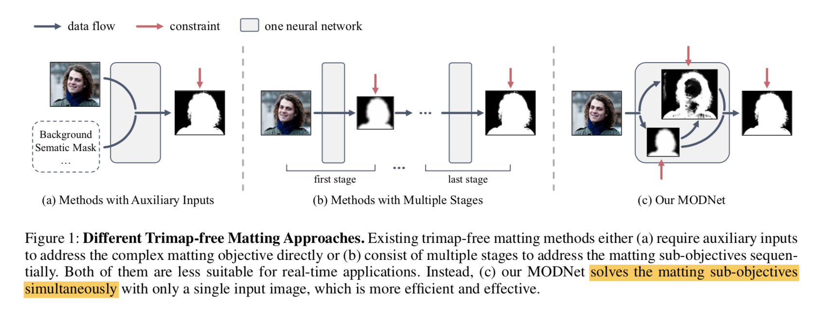
主题:query-based instance segmentation
Sparse Instance Activation for Real-Time Instance Segmentation
动机
- previous instance methods relies heavily on detection results
- this paper
- use a sparse set of instance activation maps:稀疏set作为前景目标的ROI
- aggregate the overall mask feature & instance-level feature
- avoid NMS
- 性能 & 精度
- 40 FPS
- 37.9AP on COCO
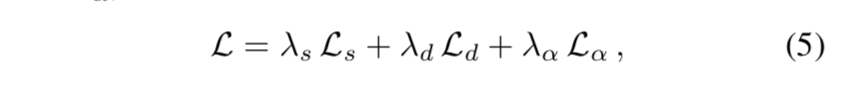
论点
两阶段methods的limitations
- dense anchors make redundant proposals伴随了heavy burden of computation
- multi-scale further aggravate the issue
- ROI-Align没法部署在终端/嵌入式设备上
- 后处理排序/NMS也耗时
this paper
- propose a sparse set called Instance Activation Maps(IAM)
- motivated by CAM
- 通过instance-aware activation maps对全局特征加权就可以获得instance-level feature
- label assignment
- use DETR‘s bipartitie matching
- avoid NMS
- propose a sparse set called Instance Activation Maps(IAM)
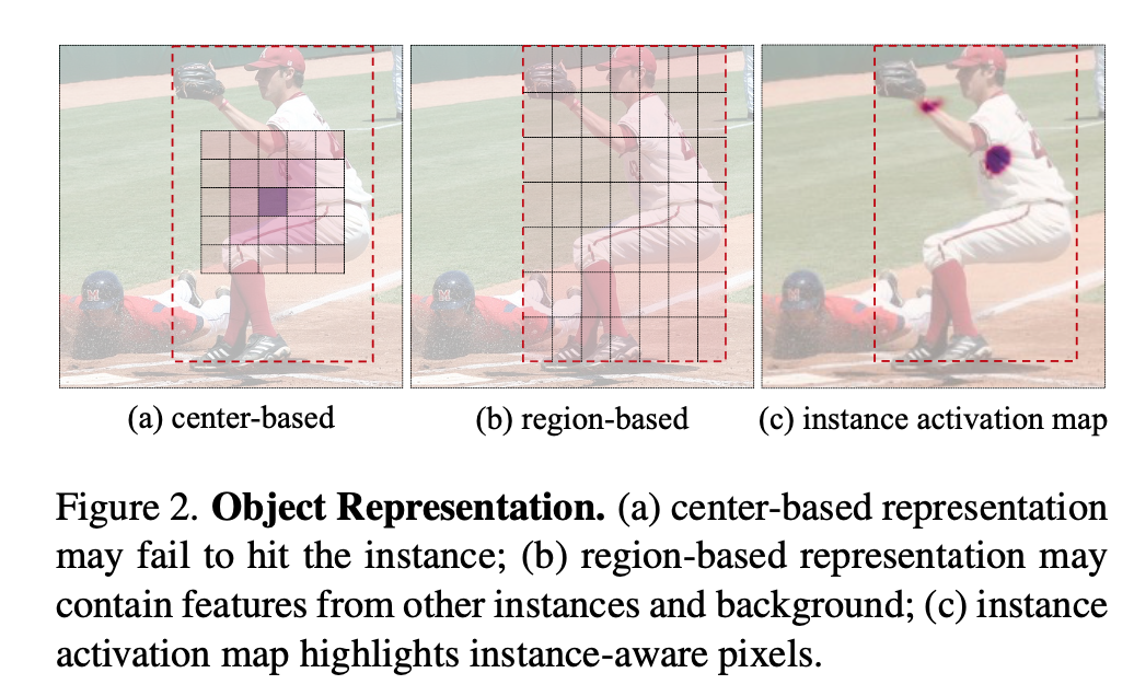
object representation对比
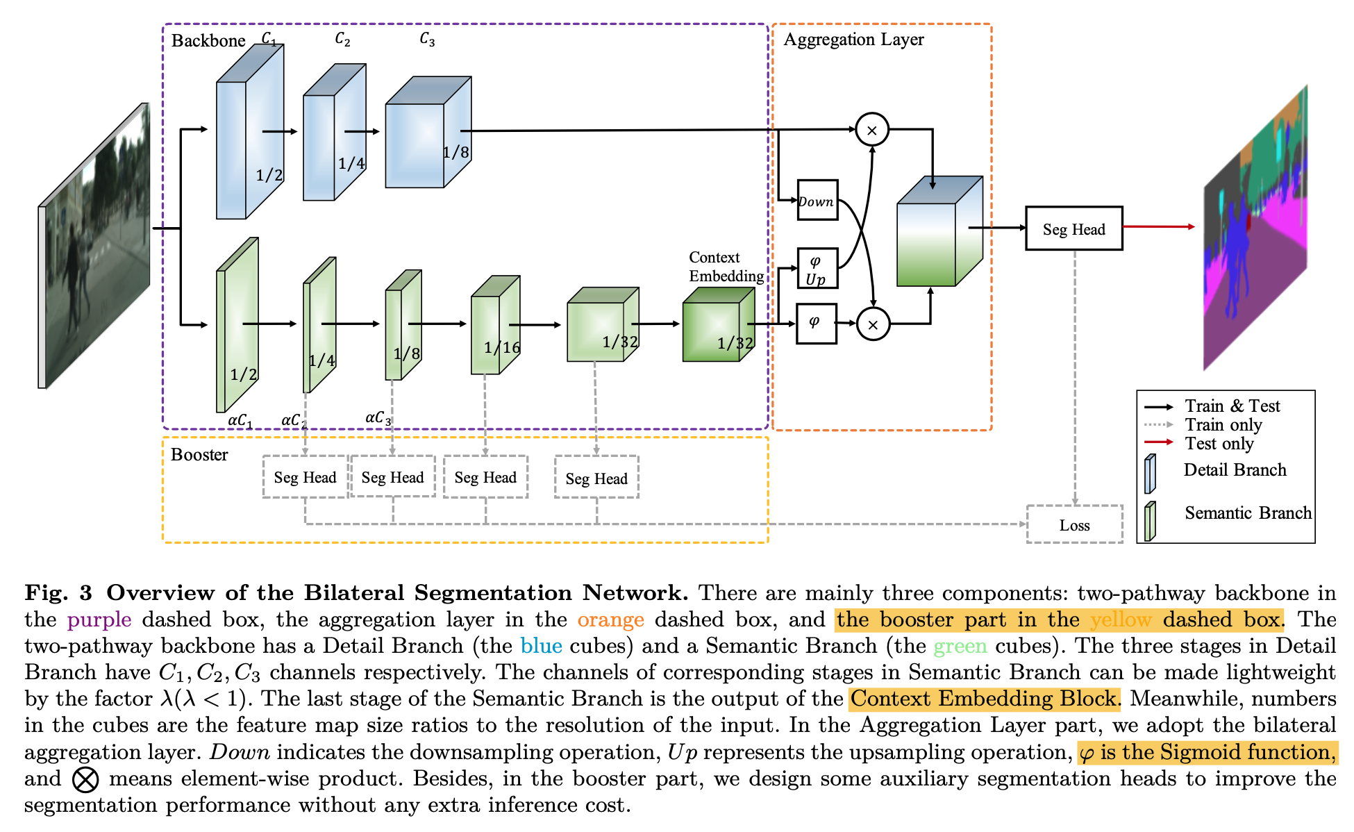
方法
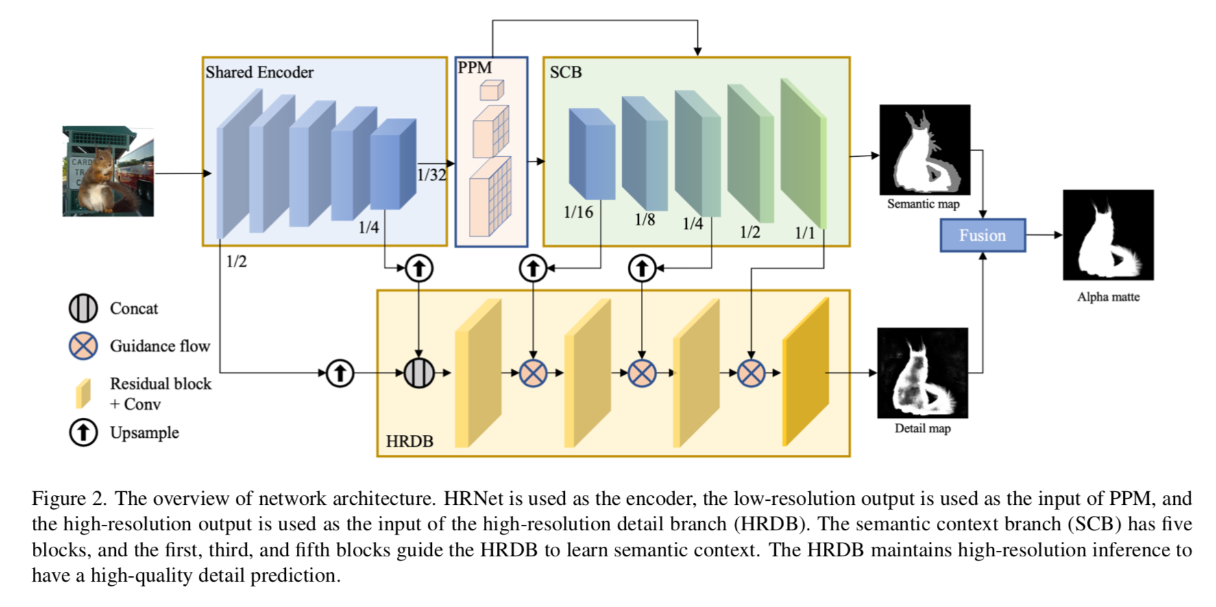
- overview
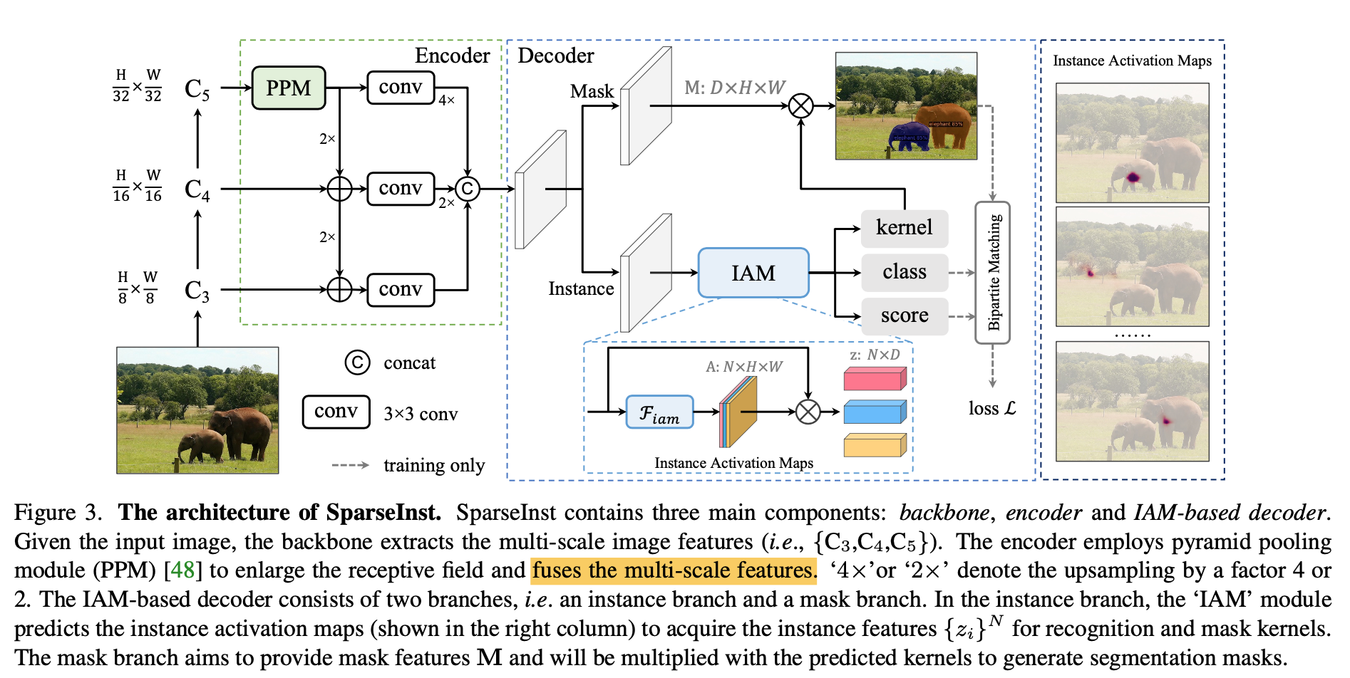
- backbone:拿到x8/x16/x32的C3/C4/C5特征
- encoder:feature pyramid,bottleneck用了PPM扩大感受野,然后bottom-up FPN,然后merge multi-scale feature to achieve single-level prediction
- IAM-based decoder:
- mask branch:provide mask features $M: D \times H \times W$
- instance branch:provide instance activation maps $k: N\times H \times W$ to further acquire recognition kernels $z: N\times D$
- IAM-based decoder
- 首先两个分支都包含了 a stack of convs
- 3x3 conv
- channel = 256
- stack=4
- location-sensitive features
- $H \times W \times 2$的归一化坐标值
- concat到decoder的输入上
- enhance instance的representation
- instance activation maps
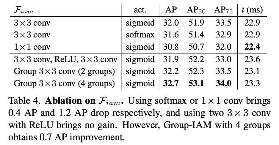
- IAM用3x3conv+sigmoid:region proposal map
- 进一步地,还有用GIAM,换成group=4的3x3conv,multiple activations per object
- 点乘在输入上,得到instance feature,$N\times D$的vector
- 然后是三个linear layer,分别得到classification/objectness score/mask kernel
- IOU-aware objectness
- 拟合pred mask和gt mask的IoU,用于评价分割模型的好坏
- 主要因为proposal大多是负样本,这种不均衡分布会拉低cls分支的精度,导致cls score和mask分布存在misalignment
- inference阶段,最终使用的fg prob是$p=\sqrt{cls_prob, obj_score}$
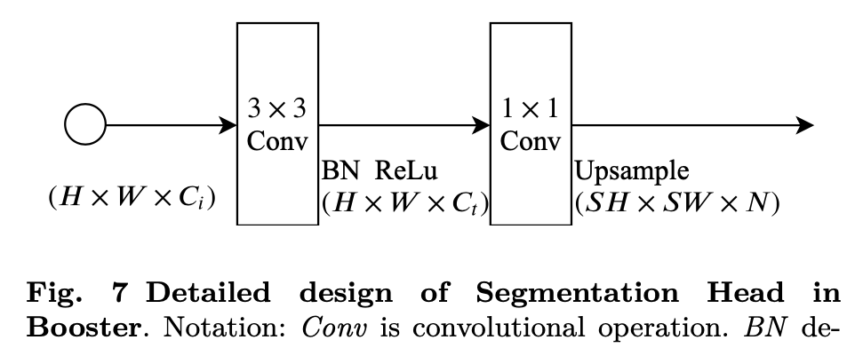
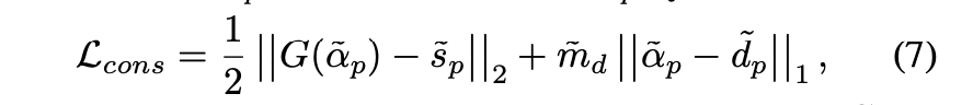
- mask head
- given instance features $w_i \in R^{1D}$and mask features $M\in R^{DHW}$
- 直接用矩阵乘法:$m_i = w_i \cdot M$
- 最后upsample到原始resolution
- 首先两个分支都包含了 a stack of convs
- matching loss
- bipartite matching
- dice-based cost
- $C(i,k)=p_i[cls_k]^{1-\alpha} * dice(m_i,gt_k)^\alpha$
- $\alpha = 0.8$
- dice用原始形式:$dice(x,y)=\frac{2 \sum x*y}{\sum x^2 + \sum y^2}$
- Hungary algorithm: scipy
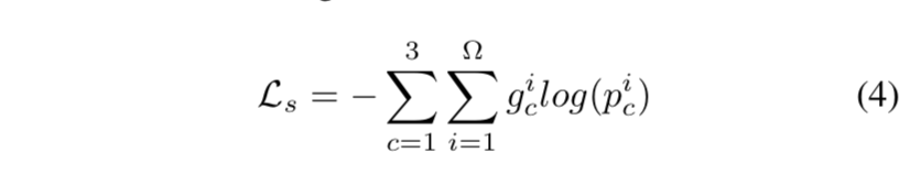
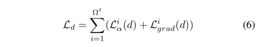
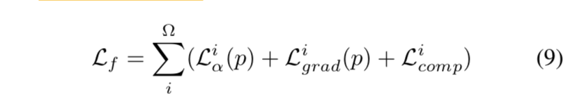
- weighted sum of
- loss cls:focal loss
- loss obj:bce
- loss mask:bce + dice
- bipartite matching
- overview
实验
dataset
- COCO 2017:118k train / 5k valid / 20k test
metric
- AP:mask的average precision
- FPS:frames per second,在Nvidia 2080 Ti上,没有使用TensorRT/FP16加速
training details
- 8卡训练,总共64 images per-mini-batch
- AdamW:lr=5e-5,wd=1e-4
- train 270k iterations
- learning rate:divided by 10 at 210k & 250k
- backbone:用了ImageNet的预训练权重,同时frozenBN
- data augmentaion:random flip/scale/jitter,shorter side random from [416,640],longer side<=864
- test/eval:use shorter size 640
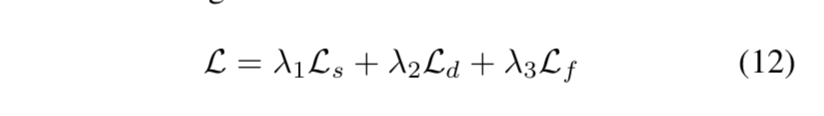
- loss weights:cls weight=2,dice weight=2,pixel bce weight=2,obj weight=1,后面实验发现提高pixel bce weight到5会有些精度gain
- proposals:N=100
results
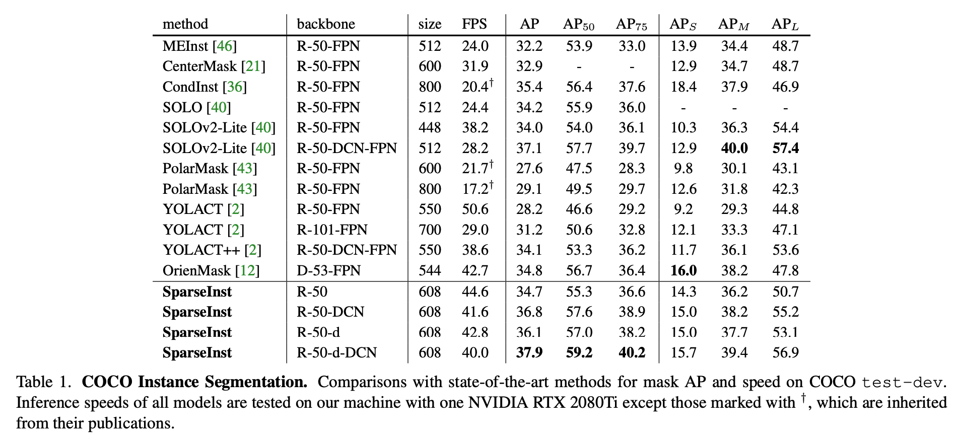
backbone主要是ResNet50
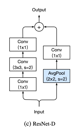
ResNet-d:bag-of-tricks paper里面的一个变种,resnet在stage起始阶段进行下采样,变种将下采样放在block里面,residual path用stride2的3x3 conv,identity path用avg pooling + 1x1 conv
ResNet-DCN:参考的是deformable conv net v2,将最后一个卷积替换成deformable conv
在数据处理上,增加了random crop,以及large weight decay(0.05),为了和竞品对齐
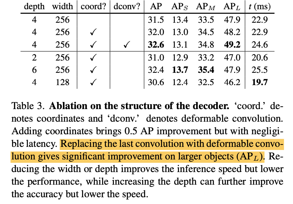
ablation on coords / dconv
ablation on FIAM:kernel size/n convs/activations / group conv