papers
[survey 2023] Diffusion Models: A Comprehensive Survey of Methods and Applications
[VAE]
[DDPM 2020] Denoising Diffusion Probabilistic Models
[LDMs 2022] High-Resolution Image Synthesis with Latent Diffusion Models
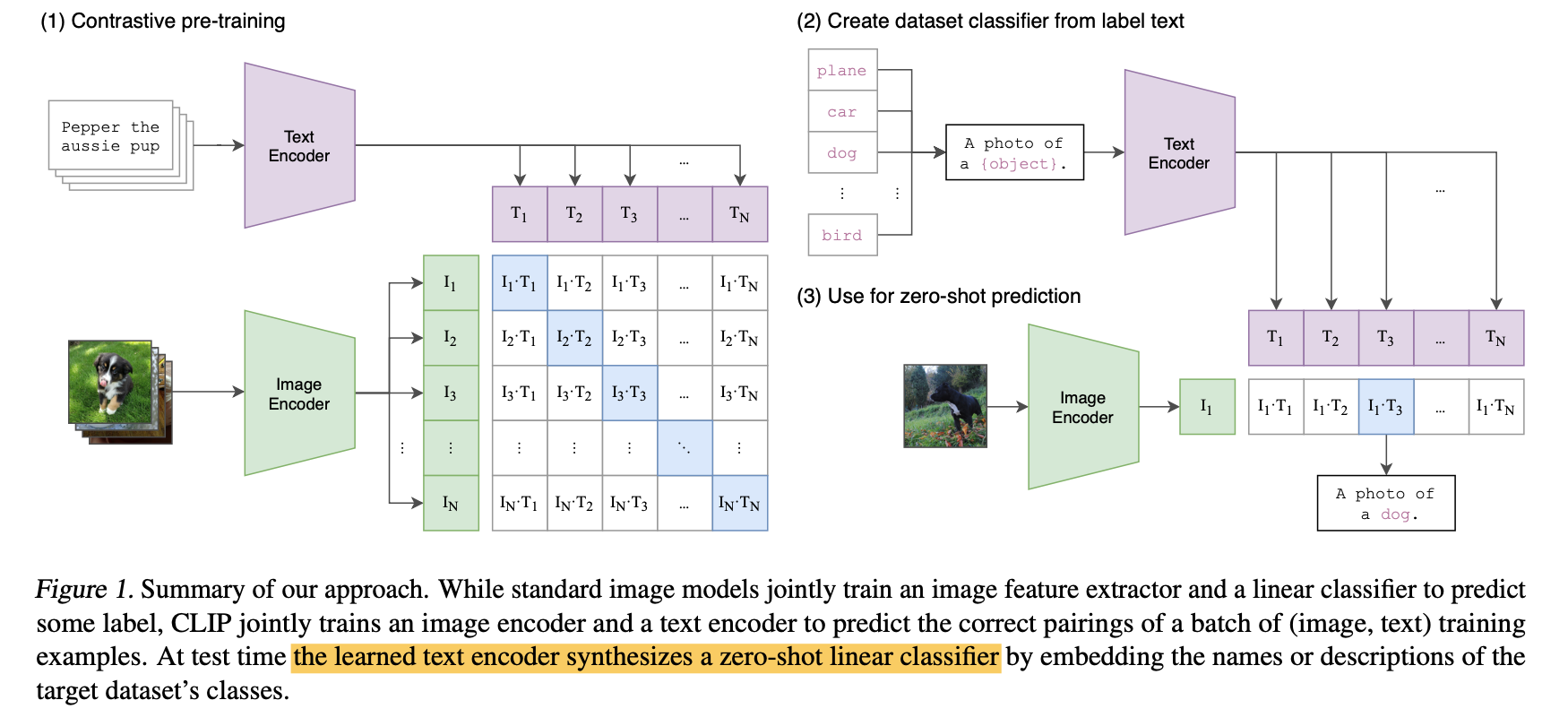
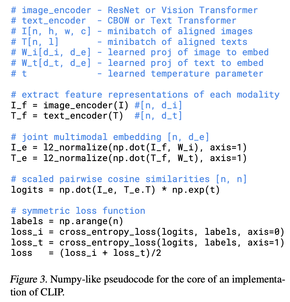
aigc Text-to-Image 大模型
Stable Diffusion
DALLE
GLIDE
微调方式
- ControlNet
- Textual Inversion
- Hypernetworks
- Lora
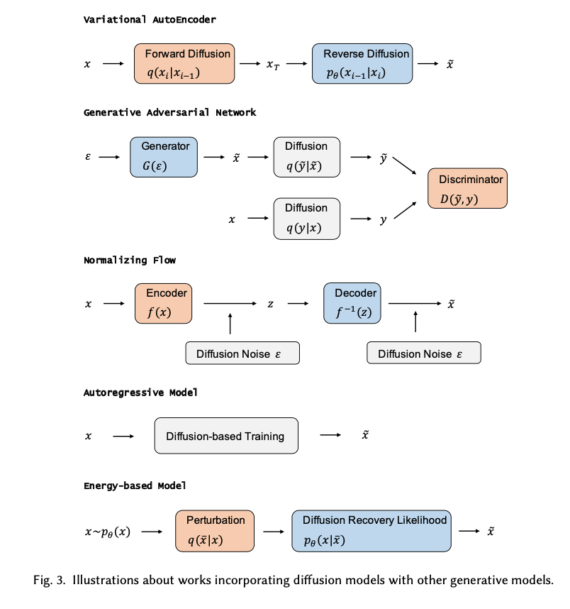
其他生成模型:
GAN
VAE
Autoregressive model
Normalizing flow
Energy-based model
Vision Tasks
- repaint:图像补全修复
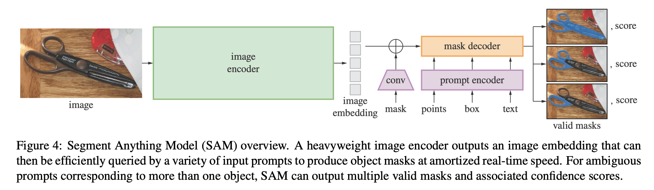
- GLIDE:文本到图像的生成
生成式建模的basic idea:正向扩散来系统地扰动数据中的分布,然后通过学习反向扩散过程恢复数据的分布
有监督的生成模型与判别模型
- 有监督学习是根据样本和标签{X,Y}去学习一个模型:$Y=f(X)$ / $p(Y|X)$,根据监督方式又分为判别模型和生成模型
- 判别模型:直接对条件概率分布建模,监督给定X预测出的Y的质量,来拟合真实分布,所有的有监督的回归、分类等模型都是判别模型
- 生成模型:建模联合概率分布$p(X,Y)$,间接计算后验概率,常见方法有朴素贝叶斯(Naive Bayes)、混合高斯模型(GMM)、隐马尔科夫模型(HMM)、GAN的生成器
无监督的生成模型
- 对输入样本X的分布建模$p(X)$,希望产生与训练集同分布的新样本
- 概率模型的输出接近X的真实分布,就可以从概率模型中采样来“生成”样本了
极大似然估计
极大似然估计是对概率模型参数进行估计的一种方法
假设训练数据服从$P_{data}(X)$,生成模型的输出分布为$P_g(X,\theta)$,可以得到关于模型参数$\theta$的函数,$L(\theta) = \Pi_i^N p_g(x_i,\theta)$
- 最好的$\theta$下产生数据集中的所有样本的概率是最大的,$\theta = argmax L(\theta)$
- 为了避免多个概率的乘积发生数值下溢问题,采用对似然函数取对数的形式,$\theta = argmax\ log(L(\theta))$
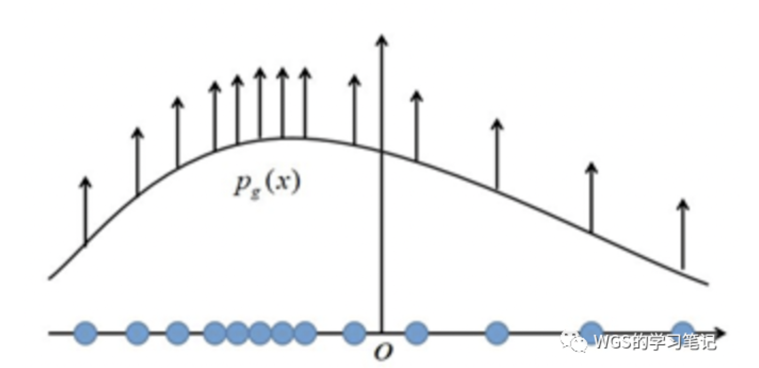
使用极大似然估计时,每个样本都希望拉高它所对应的模型概率值,但是所有样本的概率密度总和为1,一个样本点的概率密度函数值被拉高将不可避免的使其它点的函数值被拉低,最终达到一个相对平衡的状态
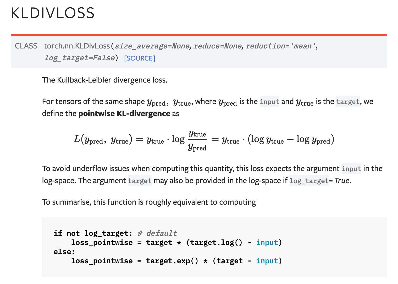
也可以直接建模成预测分布和真实分布的KL散度
- $\theta = argmax\ D_{KL}(p_{data} | p_g) = argmax \ p_g (log\ p_{data}-log\ p_g) = argmax \ log\ p_g $
- 和上面的形式一样
VAE:变分自编码器
V:Variational,变分推断
AE:Auto-Encoder
- encoder-decoder形式的重建模型
- encode:从输入x得到Latent Variable z
- decode:从隐变量z重建x
- 重建loss就是重构像素点误差,可以用MSE
- AE的局限是泛化性,仅根据已有分布重建,latent space太窄了,随机采样的latent code就是乱码了,这种性质其实很适合异常检测(GANomaly)
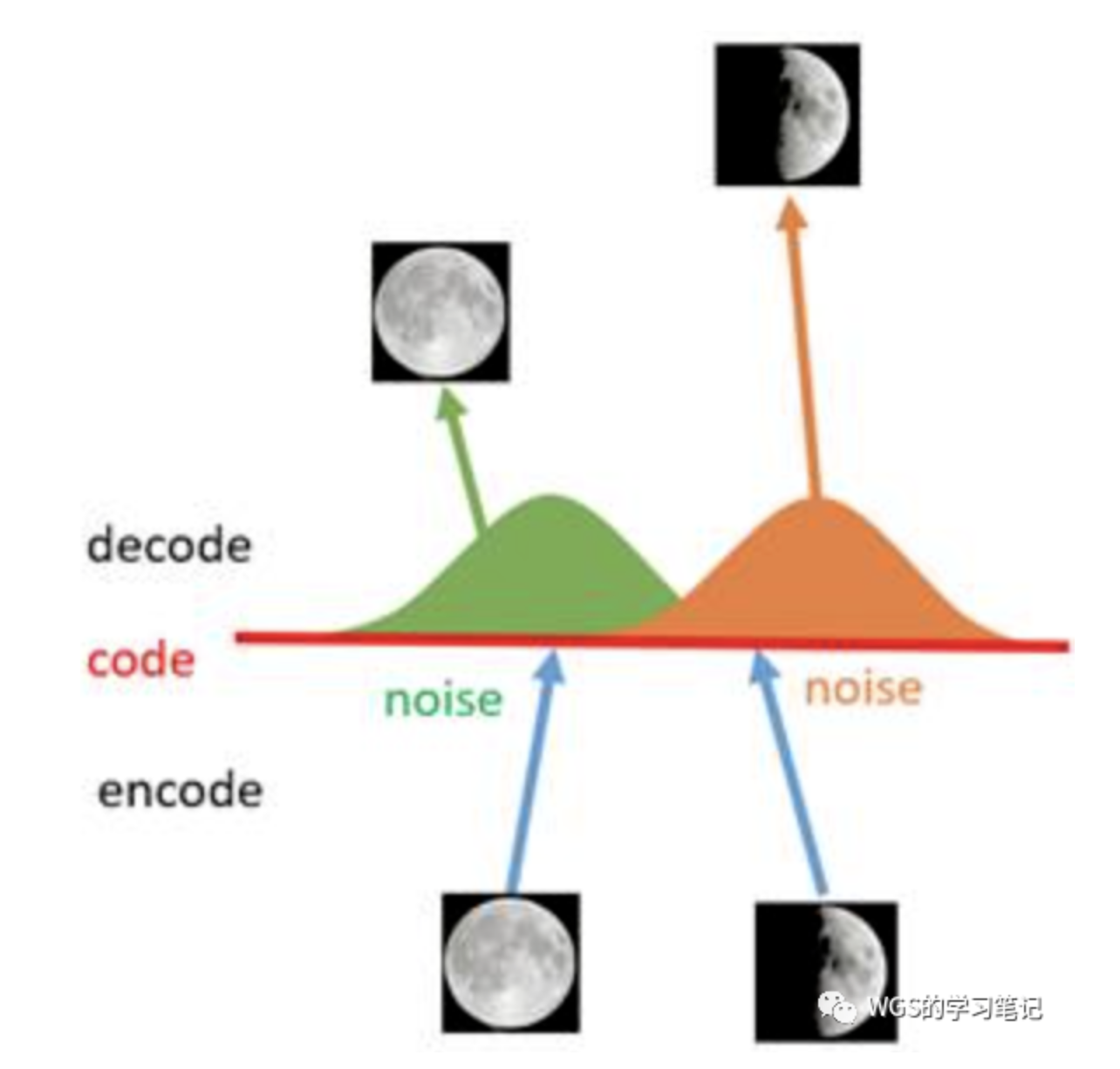
于是想到在latent code上面添加噪声,扩展latent space,一个直观的做法就是将latent code扩展成一个高斯分布,真实编码附近有一个高的概率值,远的地方概率越来越低,将一个单点扩展到整个空间
- encoder-decoder形式的重建模型
VAE
- encoder的输出不再是隐向量z,而是一个概率分布,用均值m和方差v来建模,除此以外还添加额外的高斯噪声e,间接得到latent code $z=exp(v)*e+m$
loss包含重建loss + 一个辅助loss
- 辅助loss = $e^v-(1+v) + m^2$,他对v的倒数是$e^v-1$,在v=0时取得minimum
- 防止v退化成-inf,使得VAE退化成AE
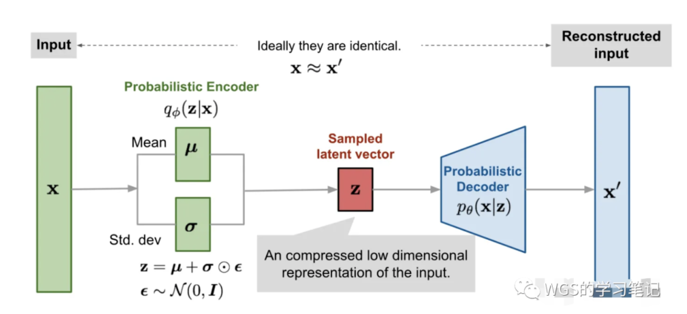
最终我们得到了一个decoder,只要我们在给定input的latent分布周围随机采样,就能得到类似input的样本
DDPM
扩散模型包括 前向扩散过程 和 反向去噪过程(采样),前向阶段对图像逐步施加噪声,直至图像被破坏变成完全的高斯噪声,然后在反向阶段学习从高斯噪声还原为原始图像的过程,最终我们可以得到一个从纯噪声生成图片的模型
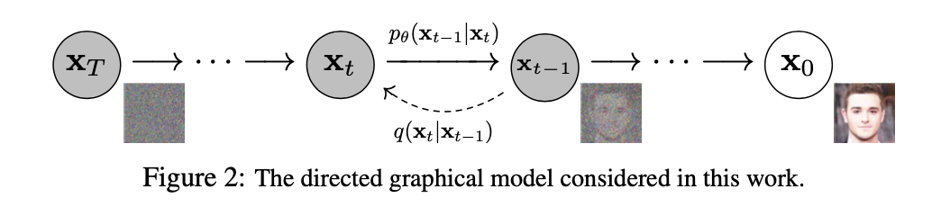
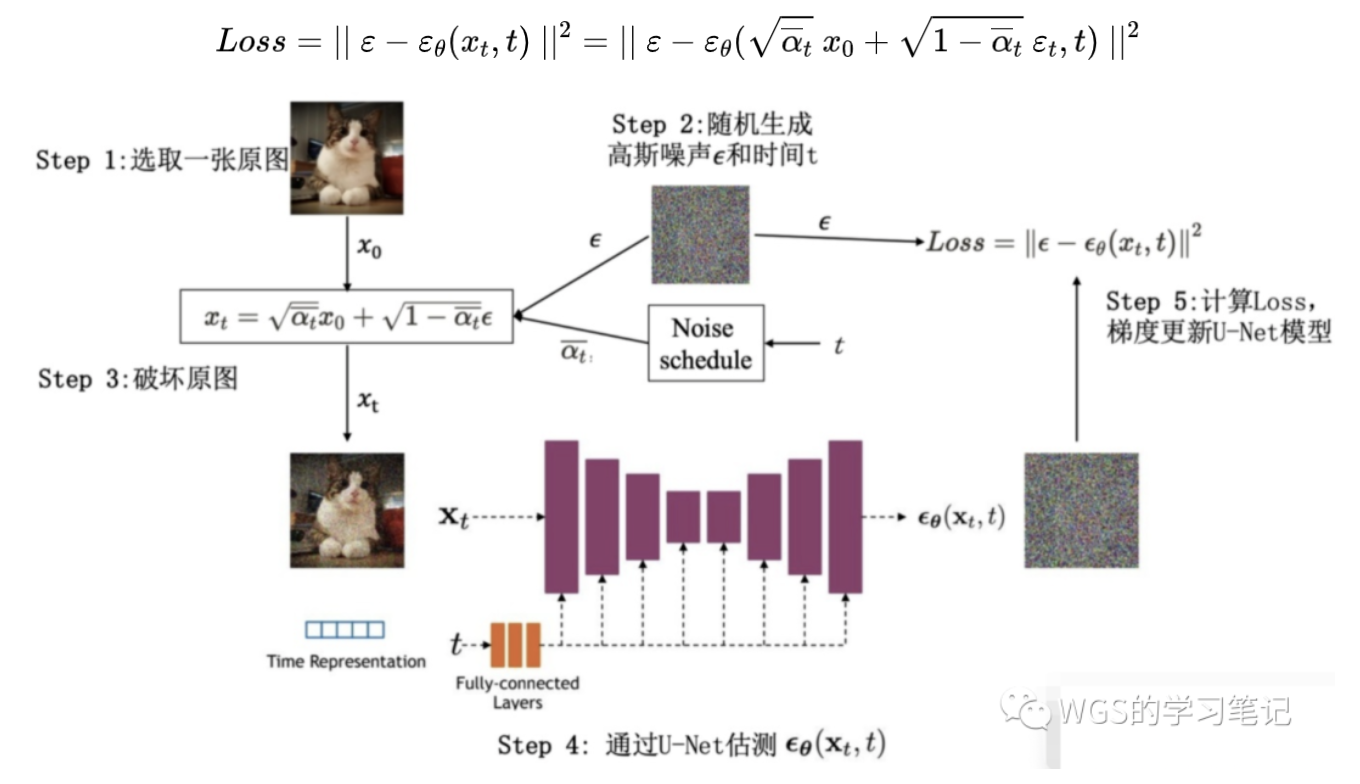
前向过程(扩散)
- 逐步向真实图片添加噪声最终得到一个纯噪声
- $x_t = \sqrt {\alpha_t} x_{t-1} + \sqrt {1-\alpha_t} \varepsilon_t$
- $\varepsilon_t$是满足正态分布的随机噪声
- $\sqrt {\alpha_t}$是图片权重,1-*是噪声权重
- $\alpha_t = 1-\beta_t$是固定的已知函数,可以直接获得的,$\beta$通常很小,accumulate $\alpha$ 逐渐变小
- $\overline \alpha = \Pi_i^t \alpha_i$ 此前所有$\alpha$的累积
- $x_t = \sqrt {\overline \alpha_t} x_{0} + \sqrt {1-\overline \alpha_t} \varepsilon_t$
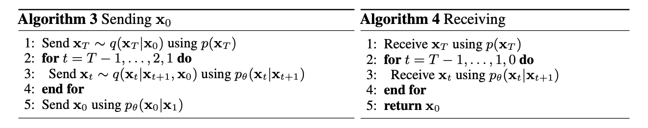
反向过程(去噪)
- 训练网络去分解每一步的噪声,Unet,得到$\varepsilon_{\theta}(x_t,t)$
- target是使预测噪声与真实噪声接近
使用模型
使用一个随机噪声,以及trained Unet噪声模型,逐步还原成一张图片
diffusion models的缺点
- 去噪过程非常耗时,并且非常消耗内存
- 因为训的是原始图片,训练的极其缓慢,LDM的改进办法就是将训练放在latent space,用预训练的大模型将原图投影到latent space
Latent Diffusion Models
将训练搬到了latent space
支持general consitioning inputs:text / bbox,用cross-attention实现多模态信息的注入
overview
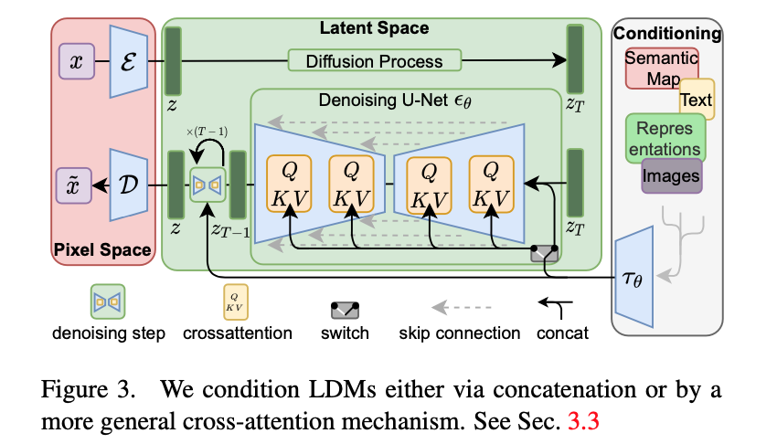
- VAE:$E$ 是encoder,用原图编码到latent space,$D$是decoder,将生成的z解码到像素space
- Condition-Encoder:编码多模态信息,text的话就用bert/clip
- UNet with cross attn:cross attn融入condition信息,指导图像生成
- ResBlock
- 输入是latent feature和timestep_embedding
- timestep_embedding是将timestep用positional embedding类似的编码方式得到的
- SpatialTransformer
- standard transformer block:self attn - cross attn - ffn
- ResBlock
- Stable Diffusion:https://jalammar.github.io/illustrated-stable-diffusion/
- deeplearning.AI:https://learn.deeplearning.ai/diffusion-models
- DDIM
- sampling is slow,DDIM faster the process by skiping timesteps
- sampling in latent space z