综述
papers
[R-CNN] R-CNN: Rich feature hierarchies for accurate object detection and semantic segmentation
[SPP] SPP-net: Spatial Pyramid Pooling in Deep Convolutional Networks for Visual Recognition
[Fast R-CNN] Fast R-CNN: Fast Region-based Convolutional Network
[Faster R-CNN] Faster R-CNN: Towards Real-Time Object Detection with Region Proposal Networks
[Mask R-CNN] Mask R-CNN
[FPN] FPN: Feature Pyramid Networks for Object Detection
[Cascade R-CNN] Cascade R-CNN: Delving into High Quality Object Detection
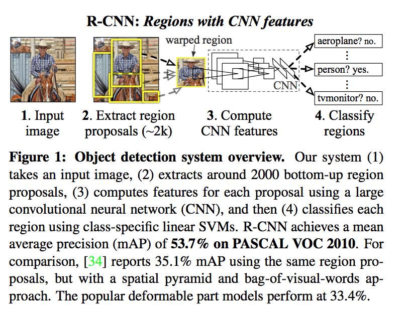
R-CNN: Rich feature hierarchies for accurate object detection and semantic segmentation
动机
- localizing objects with a deep network and training a high-capacity model with only a small quantity of annotated detection data
- apply CNN to region proposals: R-CNN represents ‘Regions with CNN features’
- supervised pre-training
- localizing objects with a deep network and training a high-capacity model with only a small quantity of annotated detection data
论点
- model as a regression problem: not fare well in practice
- build a sliding-window detector: have to maintain high spatial resolution
- what we do: our method gener- ates around 2000 category-independent region proposals for the input image, extracts a fixed-length feature vector from each proposal using a CNN, and then classifies each region with category-specific linear SVMs
- conventional solution to training a large CNN is ‘using unsupervised pre-training, followed by supervised fine-tuning’
- what we do: ‘supervised pre-training on a large auxiliary dataset (ILSVRC), followed by domain specific fine-tuning on a small dataset (PASCAL)’
- we also demonstrate: a simple bounding box regression method significantly reduces mislocalizations
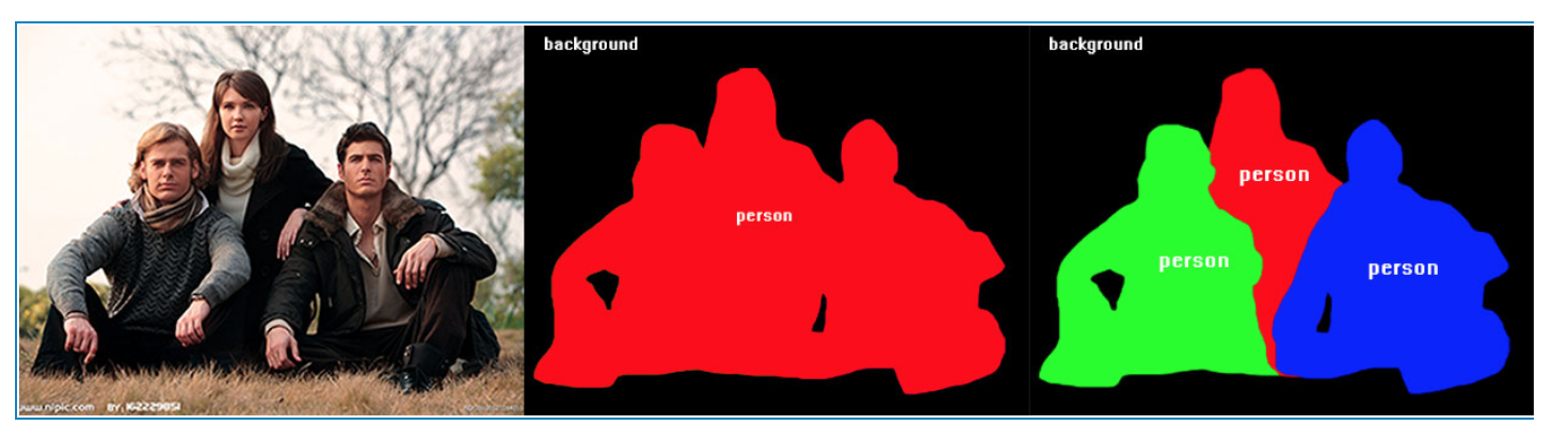
- R-CNN operates on regions: it is natural to extend it to the task of semantic segmentation
要素
- category-independent region proposals
- a large convolutional neural network that extracts a fixed-length feature vector from each region
a set of class-specific linear SVMs
方法
Region proposals: we use selective search
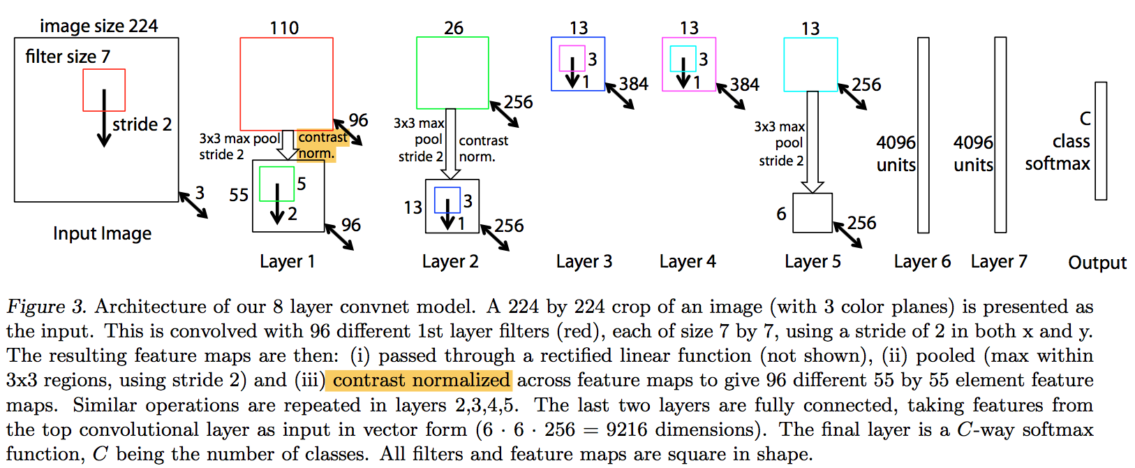
Feature extraction: we use Krizhevsky CNN, 227*227 RGB input, 5 convs, 2 fcs, 4096 output
- we first dilate the tight bounding box (padding=16)
then warp the bounding box to the required size (各向异性缩放)
Test-time detection:
- we score each extracted feature vector using the SVM trained for each class
- we apply a greedy non-maximum suppression (for each class independently)
- 对留下的这些框进行canny边缘检测,就可以得到bounding-box
- (then B-BoxRegression)
Supervised pre-training: pre-trained the CNN on a large auxiliary dataset (ILSVRC 2012) with image-level annotations
Domain-specific fine-tuning:
- continue SGD training of the CNN using only warped region proposals from VOC
- replace the 1000-way classification layer with a randomly initialized 21-way layer (20 VOC classes plus background)
- class label: all region proposals with ≥ 0.5 IoU overlap with a ground-truth box as positives, else negatives
- 1/10th of the initial pre-training rate
- uniformly sample 32 positive windows (over all classes) and 96 background windows to construct a mini-batch of size 128
Object category classifiers:
- considering a binary classifier for a specific class
- class label: take IoU overlap threshold <0.3 as negatives, take only regions tightly enclosing the object as positives
- take the ground-truth bounding boxes for each class as positives
unexplained:
the positive and negative examples are defined differently in CNN fine-tuning versus SVM training
CNN容易过拟合,需要大量的训练数据,所以在CNN训练阶段我们对Bounding box的位置限制条件限制的比较松(IOU只要大于0.5都被标注为正样本),svm适用于少样本训练,所以对于训练样本数据的IOU要求比较严格,我们只有当bounding box把整个物体都包含进去了,我们才把它标注为物体类别。
it’s necessary to train detection classifiers rather than simply use outputs of the fine-tuned CNN
上一个回答其实同时也解释了CNN的head已经是一个分类器了,还要用SVM分类:按照上述正负样本定义,CNN softmax的输出比采用svm精度低。
分析
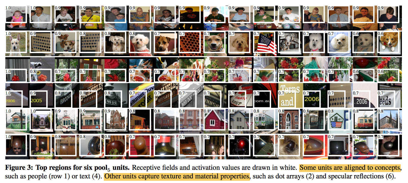
learned features:
- compute the units’ activations on a large set of held-out region proposals
- sort from the highest to low
- perform non-maximum suppression
display the top-scoring regions
Ablation studies:
- without fine-tuning: features from fc7 generalize worse than features from fc6, indicating that most of the CNN’s representational power comes from its convolutional layers
- with fine-tuning: The boost from fine-tuning is much larger for fc6 and fc7 than for pool5, suggests that pool features learned from ImageNet are general and that most of the improvement is gained from learning domain-specific non-linear classifiers on top of them
Detection error analysis:
- more of our errors result from poor localization rather than confusion
- CNN features are much more discriminative than HOG
- Loose localization likely results from our use of bottom-up region proposals and the positional invariance learned from pre-training the CNN for whole-image classification(粗暴的IOU判定前背景,二值化label,无法体现定位好坏差异)
Bounding box regression:
- a linear regression model use the pool5 features for a selective search region proposal as input
- 输出为xy方向的缩放和平移
- 训练样本:判定为本类的候选框中和真值重叠面积大于0.6的候选框
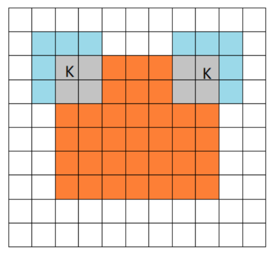
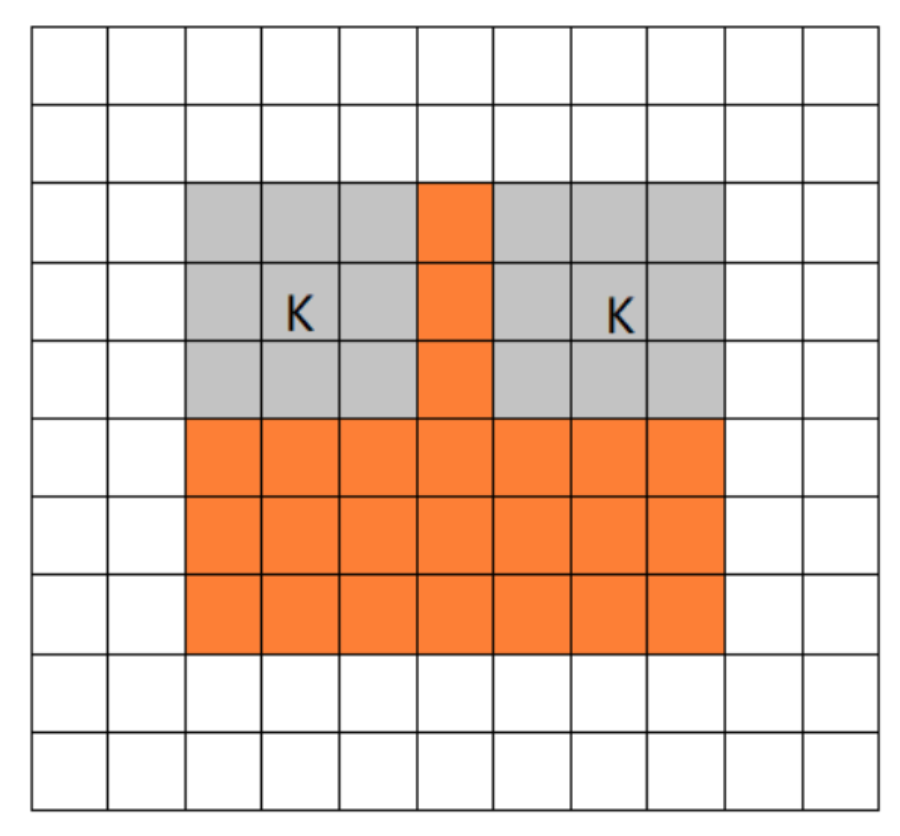
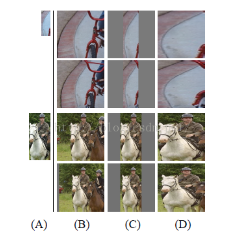
Semantic segmentation:
- three strategies for computing features:
- ‘full ‘ ignores the region’s shape, two regions with different shape might have very similar bounding boxes(信息不充分)
- ‘fg ‘ slightly outperforms full, indicating that the masked region shape provides a stronger signal
- ‘full+fg ‘ achieves the best, indicating that the context provided by the full features is highly informative even given the fg features(形状和context信息都重要)
- three strategies for computing features:
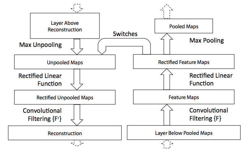
SPP-net: Spatial Pyramid Pooling in Deep Convolutional Networks for Visual Recognition
动机:
- propose a new pooling strategy, “spatial pyramid pooling”
- can generate a fixed-length representation regardless of image size/scale
- also robust to object deformations
论点:
- existing CNNs require a fixed-size input
- reduce accuracy for sub-images of an arbitrary size/scale (need cropping/warping)
- cropped region lost content, while warped content generates unwanted distortion
- overlooks the issues involving scales
- convolutional layers do not require a fixed image size, whle the fully-connected layers need to have fixed- size/length input by their definition
- by introducing the SPP layer
- between the last convolutional layer and the first fully-connected layer
- pools the features and generates fixed- length outputs
- Spatial pyramid pooling
- partitions the image into divisions from finer to coarser levels, and aggregates local features in them
- generates fixed- length output
- uses multi-level spatial bins(robust to object deformations )
- can run at variable scales
- also allows varying sizes or scales during training:
- train the network with different input size at different epoch
- increases scale-invariance
- reduces over-fitting
- in object detection
- run the convolutional layers only once on the entire image
- then extract features by SPP-net on the feature maps
- speedup
- accuracy
方法:
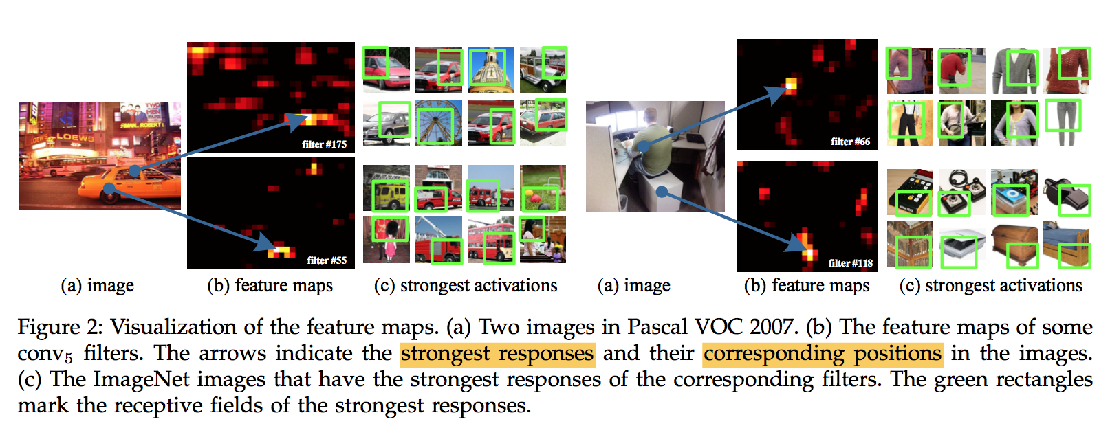
Convolutional Layers and Feature Maps
- the outputs of the convolutional layers are known as feature maps
feature maps involve not only the strength of the responses(the strength of activation), but also their spatial positions(the reception field)
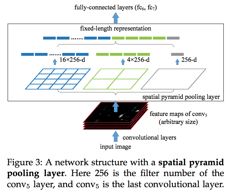
The Spatial Pyramid Pooling Layer
- it can maintain spatial information by pooling in local spatial bins
- the spatial bins have sizes proportional to the image size(k-level: 1*1, 2*2, …, k*k)
- we can resize the input image to any scale, which is important for the accuracy
the coarsest pyramid level has a single bin that covers the entire image, which is in fact a “global pooling” operation
for a feature map of $a×a$, with a pyramid level of $n×n$ bins:
Training the Network
- Single-size training: fixed-size input (224×224) cropped from images, cropping for data augmentation
- Multi-size training: rather than cropping, we resize the aforementioned 224×224 region to 180×180, then we train two fixed-size networks that share parameters by altenate epoch
- Single-size training: fixed-size input (224×224) cropped from images, cropping for data augmentation
- existing CNNs require a fixed-size input
分析
- 50 bins vs. 30 bins: the gain of multi-level pooling is not simply due to more parameters, it is because the multi-level pooling is robust to the variance in object deformations and spatial layout
- multi-size vs. single-size: multi results are more or less better than the single-size version
- full vs. crop: shows the importance of maintaining the complete content
- 50 bins vs. 30 bins: the gain of multi-level pooling is not simply due to more parameters, it is because the multi-level pooling is robust to the variance in object deformations and spatial layout
SPP-NET FOR OBJECT DETECTION
We extract the feature maps from the entire image only once
we apply the spatial pyramid pooling on each candidate window of the feature maps
These representations are provided to the fully-connected layers of the network
SVM samples: We use the ground-truth windows to generate the positive samples, use the samples with IOU<30% as the negative samples
multi-scale feature extraction:
- We resize the image at {480, 576, 688, 864, 1200}, and compute the feature maps of conv5 for each scale.
- we choose a single scale s ∈ S such that the scaled candidate window has a number of pixels closest to 224×224.
- And we use the corresponding feature map to compute the feature for this window
- this is roughly equivalent to resizing the window to 224×224
- We resize the image at {480, 576, 688, 864, 1200}, and compute the feature maps of conv5 for each scale.
fine-tuning:
- Since our features are pooled from the conv5 feature maps from windows of any sizes
- for simplicity we only fine-tune the fully-connected layers
- Since our features are pooled from the conv5 feature maps from windows of any sizes
Mapping a Window to Feature Maps**
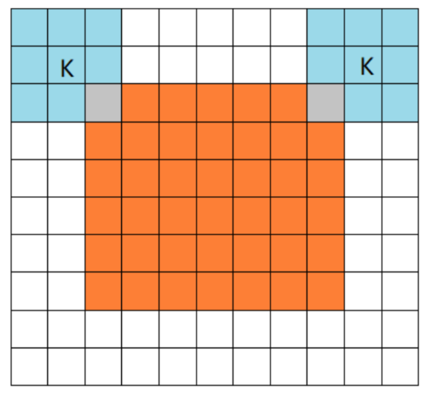
we project the corner point of a window onto a pixel in the feature maps, such that this corner point in the image domain is closest to the center of the receptive field of that feature map pixel.
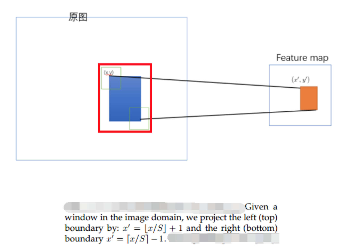
确定原图上的两个角点(左上角和右下角),映射到 feature map上的两个对应点,使得映射点$(x^{‘}, y^{‘})$在原始图上感受野(上图绿色框)的中心点与$(x,y)$尽可能接近。
Fast R-CNN: Fast Region-based Convolutional Network
动机
- improve training and testing speed
- increase detection accuracy
论点
- current approaches train models in multi-stage pipelines that are slow and inelegant
- R-CNN & SPPnet: CNN+SVM+bounding-box regression
- disk storage: features are written to disk
- SPPnet: can only fine-tuning the fc layers, limits the accuracy of very deep networks
- task complexity:
- numerous candidate proposals
- rough localization proposals must be refined
- We propose:
- a single-stage training algorithm
- multi-task: jointly learns to classify object proposals and refine their spatial locations
- current approaches train models in multi-stage pipelines that are slow and inelegant
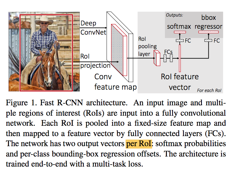
要素
- input: an entire image and a set of object proposals
- convs
- a region of interest (RoI) pooling layer: extracts a fixed-length feature vector from the feature map
- fcs that finally branch into two sibling output layers
multi-outputs:
- one produces softmax probability over K+1 classes
- one outputs four bounding-box regression offsets per class
方法
RoI pooling
- an RoI is a rectangular window inside a conv feature map, which can be defined by (r, c, h, w)
- the RoI pooling layer converts the features inside any valid RoI into a small feature map with a fixed size H × W
- it is a special case of SPPnet when there is only one pyramid level (pooling window size = h/H * w/W)
Initializing from pre-trained networks
- the last max pooling layer is replaced by a RoI pooling layer
- the last fully connected layer and softmax is replaced by the wo sibling layers + respective head (softmax & regressor)
- modified to take two inputs
Fine-tuning for detection
why SPPnet is unable to update weights below the spatial pyramid pooling layer:
原文提到feature vector来源于不同尺寸的图像——不是主要原因
feature vector在原图上的感受野通常很大(接近全图)——forward pass的计算量就很大
不同的图片forward pass的计算结果不能复用(when each training sample (i.e. RoI) comes from a different image, which is exactly how R-CNN and SPPnet networks are trained)
We propose:
takes advantage of feature sharing
mini-batches are sampled hierarchically: N images and R/N RoIs from each image
RoIs from the same image share computation and memory in the forward and backward passes
jointly optimize the two tasks
each RoI is labeled with a ground-truth class $u$ and a ground-truth bounding-box regression target $v$
the network outputs are K+1 probability $p=(p_0,…p_k)$ and K b-box regression offsets $t^k=(t_x^k, t_y^k, t_w^k,t_h^k)$
$L_{cls}$:
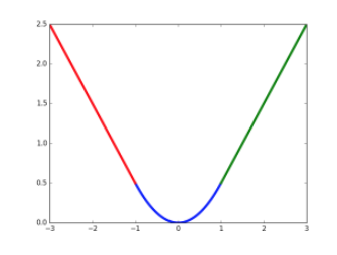
$L_{loc}$:
作者表示这种形式可以增强模型对异常数据的鲁棒性
class label: take $IoU\geq0.5$ as a foreground object, take negatives with $IoU \in [0.1,0.5)$
The lower threshold of 0.1 appears to act as a heuristic for hard example mining
Truncated SVD for faster detection
- Large fully connected layers are easily accelerated by compressing them with truncated SVD
the single fully connected layer corresponding to W is replaced by two fully connected layers, without non-linearity
The first layers uses the weight matrix $\Sigma_t V^T$(and no biases)
the second uses U (with the original biases)
分析
- Fast R-CNN vs. SPPnet: even though Fast R-CNN uses single-scale training and testing, fine-tuning the conv layers provides a large improvement in mAP
- Truncated SVD can reduce detection time by more than 30% with only a small (0.3 percent- age point) drop in mAP
- deep vs. small networks:
- for very deep networks fine-tuning the conv layers is important
- in the smaller networks (S and M) we find that conv1 is generic and task independent
- all Fast R-CNN results in this paper using models L fine-tune layers conv3_1 and up
- all experiments with models S and M fine-tune layers conv2 and up
- multi-task training vs. stage-wise: it has the potential to improve results because the tasks influence each other through a shared representation (the ConvNet)
- single-scale vs. multi-scale:
- single-scale detection performs almost as well as multi-scale detection
- deep ConvNets are adept at directly learning scale invariance
- single-scale processing offers the best tradeoff be- tween speed and accuracy thus we choose single-scale
- softmax vs. SVM:
- “one-shot” fine-tuning is sufficient compared to previous multi-stage training approaches
- softmax introduces competition, while SVMs are one-vs-rest
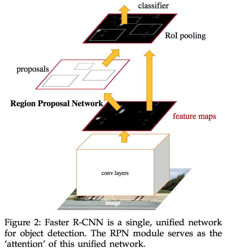
Faster R-CNN: Towards Real-Time Object Detection with Region Proposal Networks
动机
- shares the convolutional features
- merge the system using the concept of “attention” mechanisms
- sharing convolutions across proposals —-> across tasks
- translation-Invariant & scale/ratio-Invariant
论点
- proposals are now the test-time computational bottleneck in state-of-the-art detection systems
- the region proposal methods are generally implemented on the CPU
- we observe that the convolutional feature maps used by region-based detectors, like Fast R- CNN, can also be used for generating region proposals
要素
- RPN: On top of the convolutional features, we construct an RPN by adding a few additional convolutional layers that simultaneously regress region bounds and objectness scores at each location on a regular grid
- anchor: serves as references at multiple scales and aspect ratios
unify RPN and Fast R-CNN detector: we propose a training scheme that alternately fine-tuning the region proposal task and the object detection task
方法
4.1 Region Proposal Networks
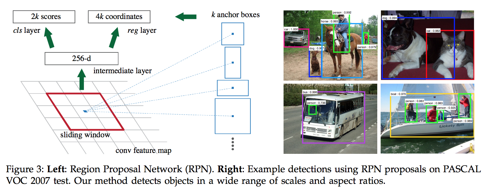
This architecture is naturally implemented with an n×n convolutional layer followed by two sibling 1 × 1 convolutional layers (for reg and cls, respectively)
conv: an n × n sliding window
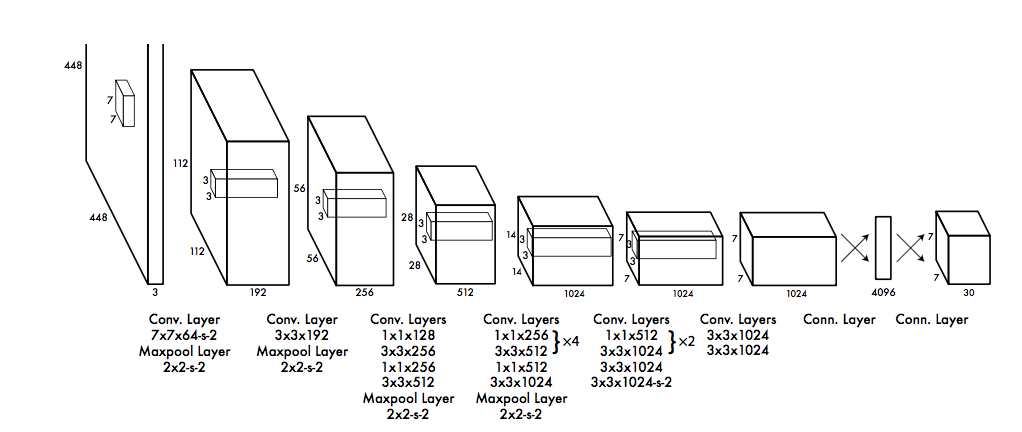
feature: 256-d for ZF(5 convs backbone) and 512-d for VGG(13 convs backbone)
two sibling fully-connected layers + respective output layer
anchors
- predict multiple region proposals: denoted as k
- the reg head has 4k outputs, the cls head has 2k outputs
- the k proposals are parameterized relative to k reference boxes————the anchors
- an anchor box is centered at the sliding window in question, and is associated with a scale and aspect ratio
- for a convolutional feature map of a size W × H , that is WHk anchors in total
class label
- positives1: the anchors with the highest IoU with a ground-truth box
- positives2: the anchors that has an IoU higher than 0.7 with any ground-truth box
- negatives: non-positive anchors if their IoU is lower than 0.3 for all ground-truth boxes
- the left: do not contribute
- ignored: all cross-boundary anchors
Loss function
similar multi-task loss as fast-RCNN, with a normalization term
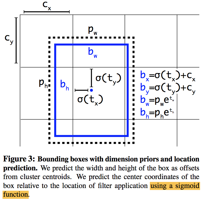
with $x,y,w,h$ denoting the box’s center coordinates and its width and height, the regression branch outputs $t_i$:
mini-batch: sampled the positive and negative anchors from a single image with the ratio of 1:1
4.2 the unified network
Alternating training
- ImageNet-pre-trained model, fine-tuning end-to-end for the region proposal task
- ImageNet-pre-trained model, using the RPN proposals, fine-tuning end-to-end for the detection task
- fixed detection network convs, fine-tuning the unique layers for region proposal
- fixed detection network convs, fine-tuning the unique layers for detection
Approximate joint training
- multi-task loss
- approximate
4.3 at training time
the total stride is 16 (input size / feature map size)
- for a typical 1000 × 600 image, there will be roughly 20000 (60*40*9) anchors in total
we ignore all cross-boundary anchors, there will be about 6000 anchors per image left for training
4.4 at testing time
we use NMS(iou_thresh=0.7), that leaves 2000 proposals per image
- then we use the top-N ranked proposal regions for detection
分析
Mask R-CNN
动机
- instance segmentation:
- detects objects while simultaneously generating instance mask
- 注意不仅仅是目标检测了
- easy to generalize to other tasks:
- instance segmentation
- bounding-box object detection
- person keypoint detection
- instance segmentation:
论点
- challenging:
- requires the correct detection of objects
- requires precisely segmentation of instances
- a simple, flexible, and fast system can surpass all
- adding a branch for predicting segmentation on Faster-RCNN
- in parallel with the existing branch for classification and regression
- the mask branch is a small FCN applied to each RoI
- Faster R- CNN was not designed for pixel-to-pixel alignment
- we propose RoIAlign to preserve exact spatial locations
- FCNs usually perform per-pixel multi-class categorization, which couples segmentation and classification
we predict a binary mask for each class independently, decouple mask(mask branch) and class(cls branch)
other combining methods are multi-stage
- our method is based on parallel prediction
- FCIS also run the system in parallel but exhibits systematic errors on overlapping instances and creates spurious edges
- segmentation-first strategies attempt to cut the pixels of the same category into different instances
- Mask R-CNN is based on an instance-first strategy
- challenging:
要素
- a mask branch with $Km^2$-dims outputs for each RoI, m denotes the resolution, K denotes the number of classes
- bce is key for good instance segmentation results: $L_{mask} = [y>0]\frac{1}{m^2}\sum bce_loss$
- RoI features that are well aligned to the per-pixel input
方法
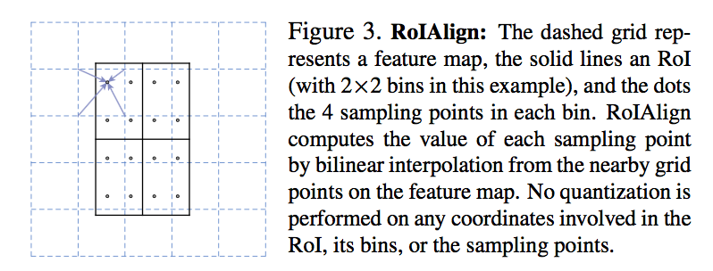
RoIAlign
- Quantizations in RoIPool: (1) RoI to feature map $[x/16]$; (2) feature map to spatial bins $[a/b]$; $[]$ denotes roundings
- These quantizations introduce misalignments
We use bilinear interpolation to avoid quantization
- sample several points in the spatial bins
- computes the value of each sampling point by bilinear interpolation from the nearby grid points on the feature map
- aggregate the results of sampling points (using max or average)
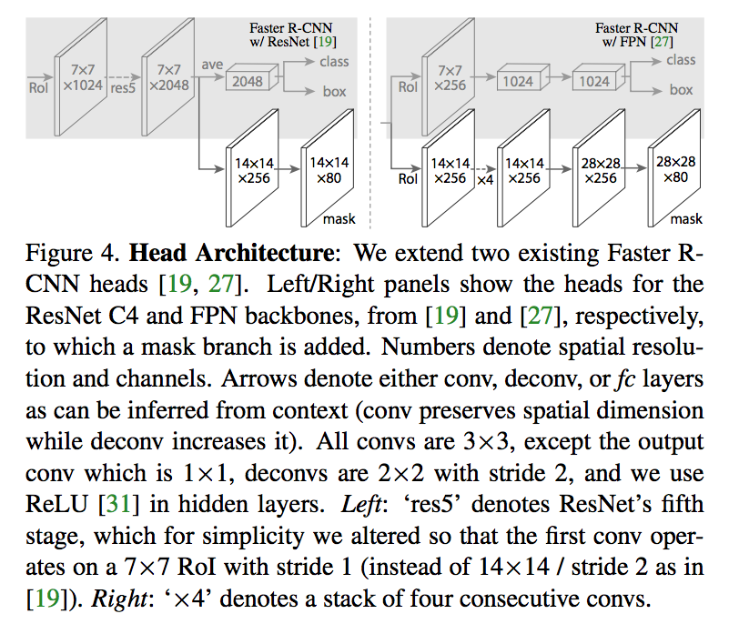
Architecture
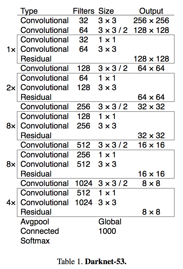
- backbone: using a ResNet-FPN backbone for feature extraction gives excellent gains in both accuracy and speed
head: use previous heads in ResNet/FPN(res5 contained in head/backbone)
Implementation Details
- positives: RoIs with IoU at least 0.5, otherwise negative
- loss: dice loss defined only on positive RoIs
- mini-batch: 2 images, N RoIs
- at training time: parallel computation for 3 branches
- at test time:
- serial computation
- proposals -> box prediction -> NMS -> run mask branch on the highest scoring 100 detection boxes
- it speeds up inference and improves accuracy
- the $28*28$ floating-number mask output is resized to the RoI size, and binarized at a threshold of 0.5
分析
- on overlapping instances: FCIS+++ exhibits systematic artifacts
- architecture: it benefits from deeper networks (50 vs. 101) and advanced designs including FPN and ResNeXt
- FCN vs. MLP for mask branch
- Human Pose Estimation
- We model a keypoint’s location as a one-hot mask, and adopt Mask R-CNN to predict K masks, one for each of K keypoint types
- the training target is a one-hot $mm$ binary mask where only a single* pixel is labeled as foreground
- use the cross-entropy loss
- We found that a relatively high resolution output ($56*56$ compared to masks) is required for keypoint-level localization accuracy
FPN: Feature Pyramid Networks for Object Detection
动机
- for object detection in multi-scale
- struct feature pyramids with marginal extra cost
- practical and accurate
- leverage the pyramidal shape of a ConvNet’s feature hierarchy while creating a feature pyramid that has strong semantics at all scales
论点
- single scale offers a good trade-off between accuracy and speed while multi-scale still performs better, especially for small objects
- featurized image pyramids form the basis solution for multi-scale
- ConvNets are proved robust to variance in scale and thus facilitate recognition from features computed on a single input scale
- SSD uses the naturely feature hierarchy generated by ConvNet which introduces large semantic gaps caused by different depths
- high-level features are low-resolution but semantically strong
- low-level features are of lower-level semantics, but their activations are more accurately localized as subsampled fewer times
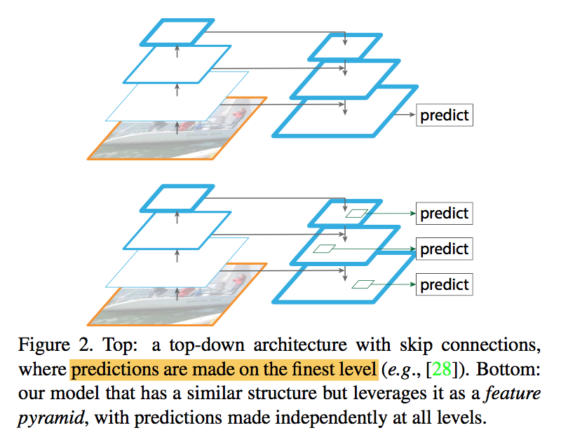
thus we propose FPN:
- combines low-resolution, semantically strong features with high-resolution, semantically weak features via a top-down pathway and lateral connections
- has rich semantics at all levels
- built from a single scale
- can be easily extended to mask proposals
- can be trained end-to- end with all scales
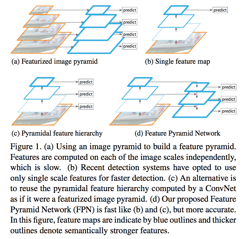
similar architectures make predictions only on a fine resolution
要素
- takes a single-scale image of an arbitrary size as input
- outputs proportionally sized feature maps at multiple levels
- structure
- a bottom-up pathway: the feed-forward computation of the backbone ConvNet
- a top-down pathway and lateral connection:
- upsampling the spatially coarser, but semantically stronger, feature maps from higher pyramid levels
- then enhance with features from the bottom-up pathway via lateral connections
- a $33$ conv is appended on each merged map *to reduce the aliasing effect of upsampling
- shared classifiers/regressors among all levels, thus using fixed 256 channels convs
- upsamling uses nearest neighbor interpolation
- low-level features undergoes a $1*1$ conv to reduce channel dimensions
- merge operation is a by element-wise addition
- adopt the method in RPN & Fast-RCNN for demonstration
方法
RPN
- original design:
- backbone Convs -> single-scale feature map -> dense 3×3 sliding windows -> head($33$ convs + 2 sibling $11$ conv branches)
- for regressor: multi-scale anchors(e.g. 3 scales 3 ratios -> 9 anchors)
- new design:
- adapt FPN -> multi-scale feature map -> sharing heads
- for regressor: set single-scale anchor for each level respectively (e.g. 5 level 3 ratios -> 15 anchors)
- sharing heads:
- vs. not sharing: similar accuracy
- indicates all levels of FPN share similar semantic levels (contrasted with naturally feature hierarchy of CNNs)
- original design:
Fast R-CNN
original design: take the ROI feature map from the output of last conv layer
new design: take the specific level of ROI feature map based on ROI area
with a $w*h$ ROI on the input image, $k_0$ refers to the target level on which an RoI with $w×h=224^2$ should be mapped into
the smaller the ROI area, the lower the level k, the finer the resolution of the feature map
分析
- RPN
- use or not FPN: boost on small objects
- use or not top-down pathway: semantic gaps
- use or not lateral connection: locations
- use or not multi-levels feature maps:
- using P2 alone leads to more anchors
- more anchors are not sufficient to improve accuracy
- Fast R-CNN
- using P2 alone is marginally worse than that of using all pyramid levels
- we argue that this is because RoI pooling is a warping-like operation, which is less sensitive to the region’s scales
Faster R-CNN
- sharing features improves accuracy by a small margin
- but reduces the testing time
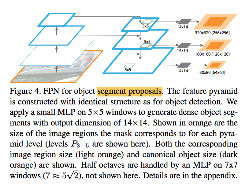
Segmentation Proposals
- use a fully convolutional setup for both training and inference
apply a small 5×5 MLP to predict 14×14 masks
- RPN
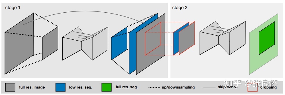
衍生应用:
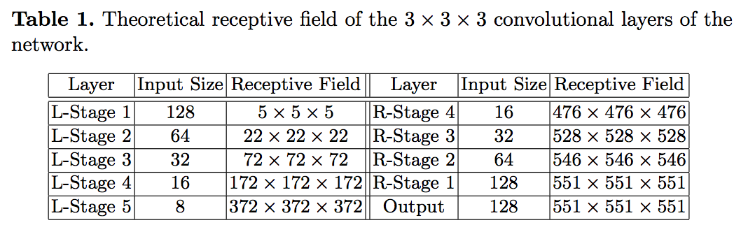
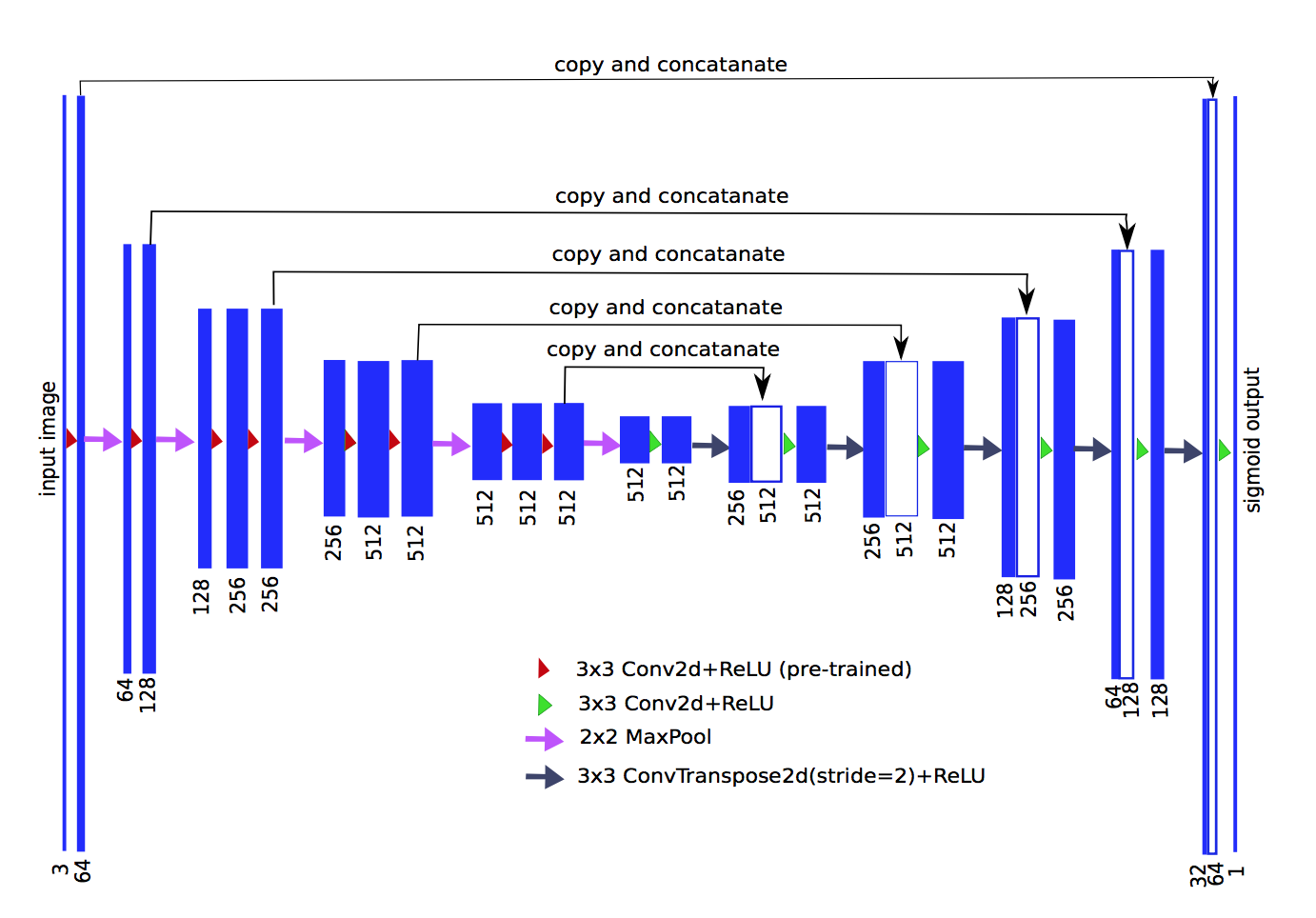
- 动机
- 3D volume detection and segmentation
- ROI / full scan
- LUNA16:lung nodules size evaluation
- 论点
- variety among nodules & similarity among non-nodules
- 方法
- use overlapping sliding windows
- use focal loss improve class result
- use IOU loss improve mask result
- use heavy augmentation
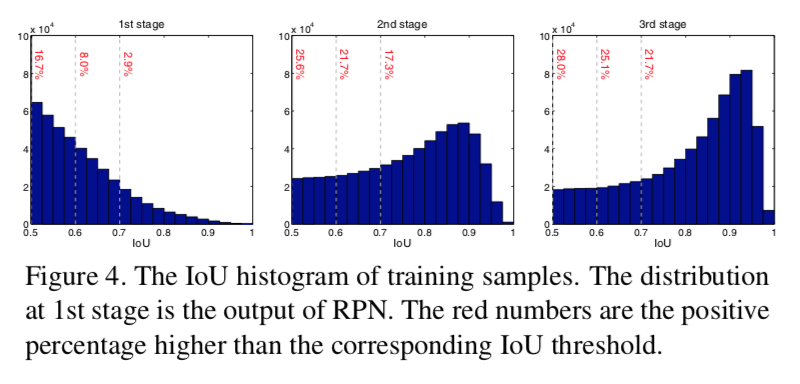
Cascade R-CNN: Delving into High Quality Object Detection
动机
- an detector trained with low IoU threshold usually produces noisy detections:低质量框issue
- 但是又不能简单地提高IoU threshold
- 正样本会急剧减少,导致过拟合
- inference-time mismatch,训练阶段只有高质量框,但是测试阶段啥质量框都有
- we propose Cascade R-CNN
- multi-stage object detection architecture
- consists of a sequence of detectors trained with increasing IoU thresholds
- trained stage by stage
- surpass all single-model on COCO
论点
- object detections two main tasks
- recognition problem:foreground/backgroud & object class
- localization problem:bounding box
- loose requirement for positives
- an low IoU thresh(0.5) is required to define positives/negatives:looss
- noisy bounding boxes:close false positives
- quality
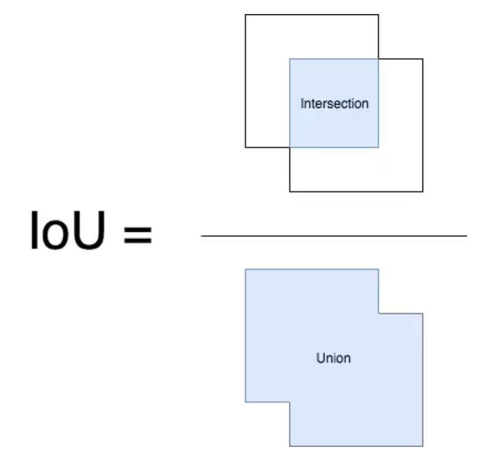
- 将一个框和gt的IoU定义为它的quality
- 将一个detector训练用的IoU thresh定义为它的quality
- detector的quality和input proposals的quality是相关的:a single detector work on a specific quality level of hypotheses
- Cascade R-CNN
- multi-stage extension of R-CNN
- sequentially more selective against close false positives
- object detections two main tasks
方法
formulation
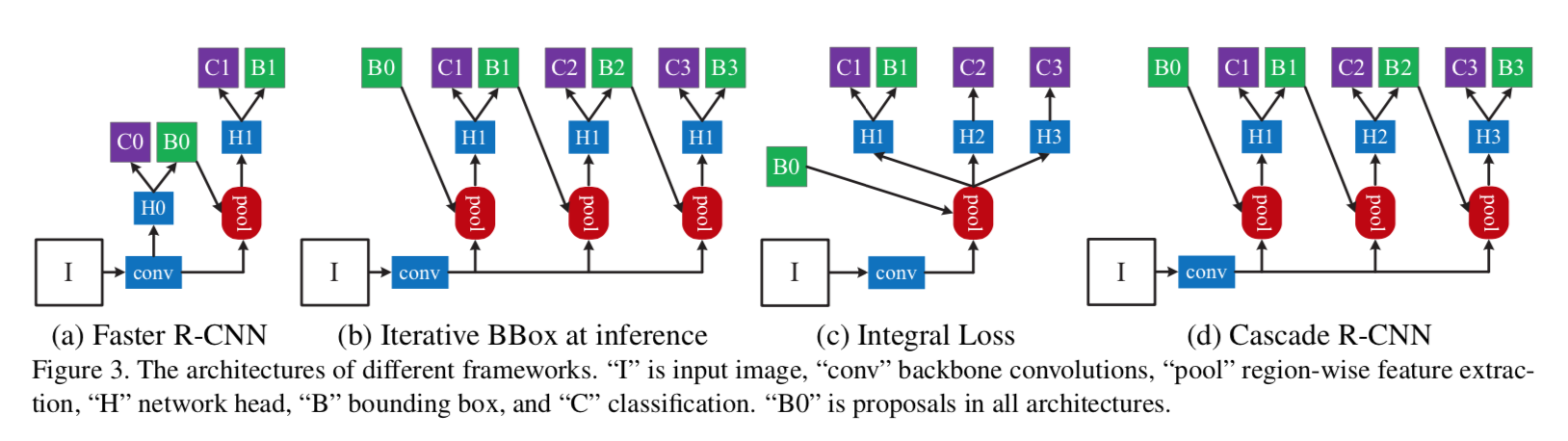
- first stage:
- proposal network H0
- applied to entire image
- second stage
- region-of-interest detection sub-network H1 (detection head)
- run on proposals
- C和B是classification score & bounding box regression
- we focus on modeling the second stage
- first stage:
bounding box regression 针对回归质量
- an image patch $x$
- a bounding box $b = (b_x, b_y, b_w, b_h)$
- use a regressor $f(x,b)$ to fit the target $g$
- use L1 loss $L_{loc}(f(x_i,b_i), g_i)$
- compute on 相对量 & std normalization
- invariant to scale and location
- results in minor adjustments on $b$:所以regression loss通常比cls loss小得多
- Iterative BBox
- a single regression step is not sufficient for accurate localization
- 所以就搞了N个一样的regression heads串联
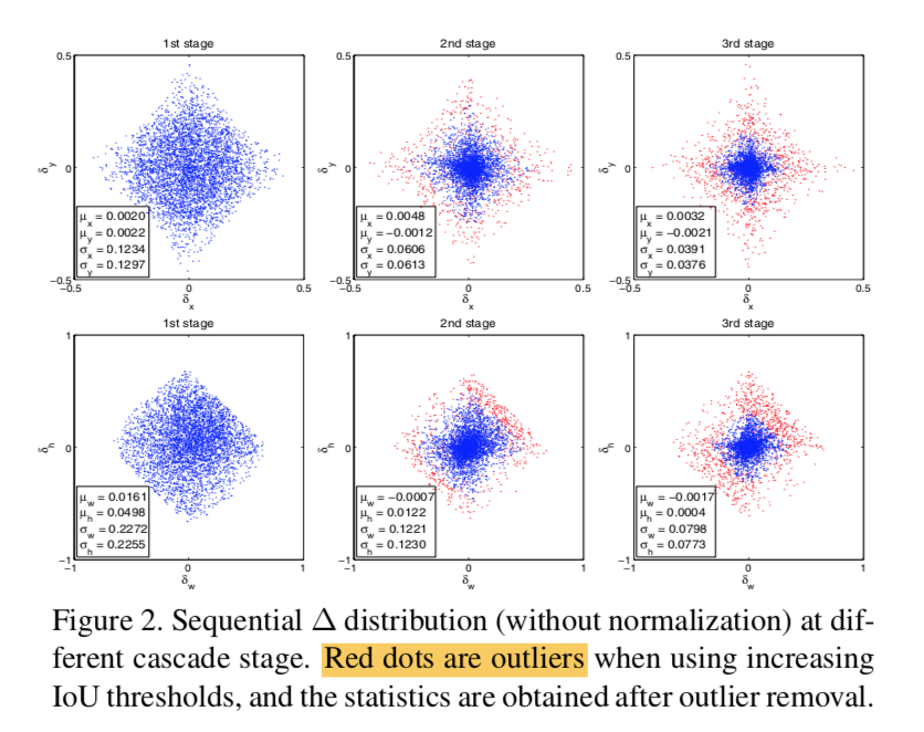
- 但还是那个问题:一个regressor只针对某一个quality level的proposals是performance optimal的,但是每个iteration以后框的distribution是剧烈变化的
- 所以迭代两次以上基本没有gain了
detection quality 针对分类质量
- an image patch x
- M foreground classes and 1 background
- use a classifier $h(x)$ to learn the target class label among M+1
- use CE $L_{cls}(h(x_i),y_i)$
- the class label is determined by IoU thresh:如果image patch和gt box的IoU大于阈值,那么这个image patch的class label就是gt box的label,否则是背景
- the IoU thresh defines the quality of a detector
- challenging
- 如果阈值调高了,positives里面包含更少的背景(高质量前景),但是样本量少
- 如果阈值低了,前景样本多了,但是内容更加diversified,更难reject close false positives
- 所以一个分类器在不同的IoU阈值下,要面临不同的问题,在inference阶段,it is very difficult to perform uniformly well over all IoU levels
- Integral loss
- 训练好几个分类器,针对不同的IoU level,然后inference阶段ensemble
- 还是没有解决高IoU阈值的那个分类器会因为样本量少过拟合的问题,而且高质量分类器在infernce阶段还是要处理所有的低质量框
Cascade R-CNN
- Cascaded Bounding Box Regression
- cascade specialized regressors
- differs from Iterative BBox
- Iterative BBox是个后处理手段,一个regressor在0.5level的boxes上面优化,然后在inference proposals上面反复迭代
- Cascade R-CNN是个resampling method,多个不同的regressor级连,训练测试同操作同分布
Cascaded Detection
- resamping manner
- keep上一阶段的positives
- 同时丢掉一些outliers
- 实现就是每个stage的IoU threshold逐渐提高
loss还是所有proposals的cls loss + 定义为前景proposals的reg loss
outliers
proposal quality
- resamping manner
- Cascaded Bounding Box Regression