Reducing the Hausdorff Distance in Medical Image Segmentation with Convolutional Neural Networks
动机
- novel loss function to reduce HD directly
- propose three methods
- 2D&3D,ultra & MR & CT
- lead to approximately 18 − 45% reduction in HD without degrading other segmentation performance criteria
论点
- HD is one of the most informative and useful criteria because it is an indicator of the largest segmentation error
- current segmentation algorithms rarely aim at minimizing or reducing HD directly
- HD is determined solely by the largest error instead of the overall segmentation performance
- HD‘s sensitivity to noise and outliers —> modified version
- the optimization diffculty
- thus we propose an “HD- inspired” loss function
方法
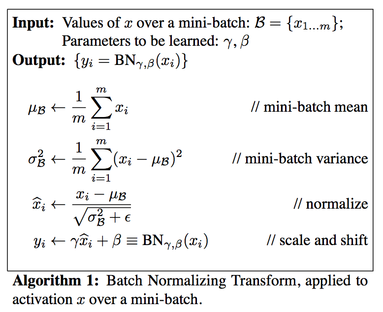
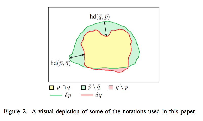
denotations
- probability:$q$
- binary mask:$\bar p$、$\bar q$
- boundary:$\delta p$、$\delta q$
single hd:$hd(\bar p, \bar q)$、$hd(\bar q, \bar p)$
based on distance transforms
distance map $d_p$:define the distance map as the unsigned distance to the boundary $\delta p$
距离场定义为:每个点到目标区域(X)的距离的最小值
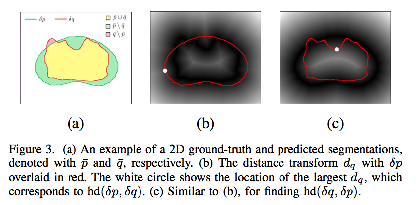
HD based on DT:
- finally have:
modified loss version of HD:
- penalizely focus on areas instead of single point
- $\alpha$ determines how strongly we penalize larger errors
- use possibility instead of thresholded value
- use $(p-q)^2$ instead of $|p-q|$
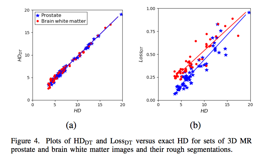
correlations
- $HD_{DT}$:Pearson correlation coefficient above 0.99
$Loss_{DT}$:Pearson correlation coefficient above 0.93
drawback
high computational cost especially in 3D
$q$ changes along with training process thus $d_q$ changes while $d_p$ remains
modified one-sided HD (OS):
HD using Morphological Operations
morphological erosion:
腐蚀操作定义为:在原始二值化图的前景区域,以每个像素为中心点,run structure element block B,如果B完全在原图内,则当前中心点在腐蚀后也是前景。
HD based on erosion:
- $HD_{ER}$ is a lower bound of the true value
- can be computed more efficiently using convolutional operations
modifid loss version:
- k successive erosions
- cross-shaped kernel whose elements sum to one followed by a soft thresholding at 0.50
correlations
- $HD_{ER}$:Pearson correlation coefficient above 0.91
- $Loss_{ER}$:Pearson correlation coefficient above 0.83
HD using circular-shaped convolutional kernel
circular-shaped kernel
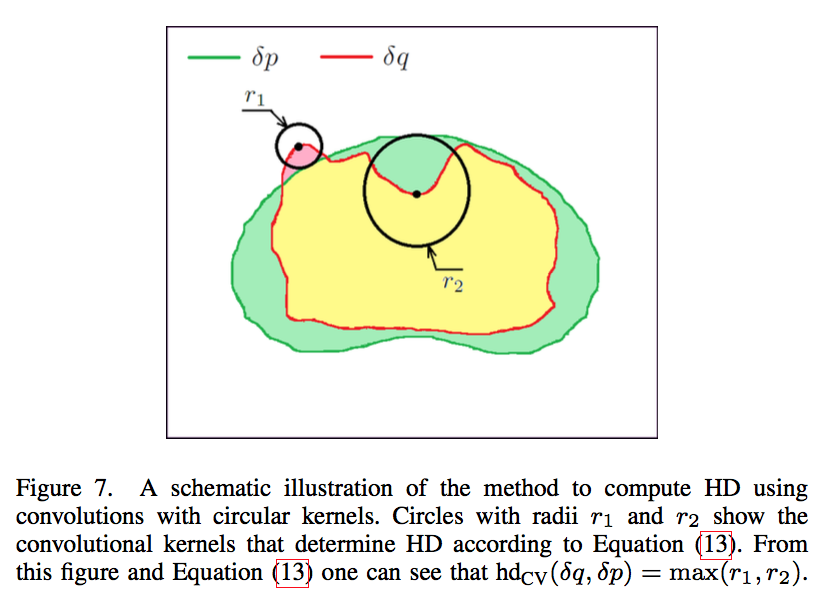
HD based on circular-shaped kernel:
- $\bar p^C$:complement 补集
- $f_h$:hard thresholding setting all values below 1 to zero
modified loss version:
- soft thresholding
correlations
- $HD_{CV}$:Pearson correlation coefficient above 0.99
- $Loss_{CV}$:Pearson correlation coefficient above 0.88
computation:
- kernel size
- $HD_{ER}$ is computed using small fixed convolutional kernels (of size 3)
- $Loss_{CV}$ require applying filters of increasing size(we use a maximum kernel radius of 18 pixels in 2D and 9 voxels in 3D)
- steps
- choose R based on the expected range of segmentation errors
- set R = {3, 6, . . . 18} for 2D images and R = {3,6,9} for 3D
- kernel size
training
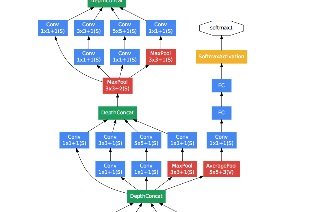
- standard Unet
- augment our HD-based loss term with a DSC loss term for more stable training
- reweight both loss after every epoch
d