MRI
T1加权相上面密度高的骨头会比较亮(就是高信号),还有脂肪和甲状腺也是高信号,水份一般都是无信号,
T2加权相里水是高信号所以水比较亮,因为很多的病变有水肿,所以T2加权相通俗可以说是看病变(毕竟比较明显),视觉直观上来看,T1看解剖,T2看病变
——怎么fusion一个case(标注只有一张)
数据集
T1、T2矢状位,T2轴状位,
关键点:基于T2矢状位的中间帧,
标注范围:从胸12(T12)腰1(L1)间的椎间盘开始,到腰5(L5)骶1(S1)间的椎间盘结束
类别:椎块有编号(T12到L5),间盘通过上下椎块的编号表示(T12-L1到L5-S1)
病灶:
 * 椎块有两类:正常V1和退行性病变V2,
 * 椎间盘有7类:正常V1,退行性改变V2,弥漫性膨出,非对称性膨出,突出,脱出,疝出V7
json结构:
- uid,dim,spacing等一些header info
- annotation:
- slice:难道不是T2矢状位的中间帧吗?
- point:关键点坐标,病灶类别,关键点类别
评估指标
distance<8mm
TP:多个命中取最近的,其余忽略
- FP:假阳性,distance超出所有gt的8mm圈圈/落进圈圈但是类别错了
- FN:假阴性,gt点没有被TP
- precision:TP/(TP+FP)
- recall:TP/(TP+FN)
- AP
- MAP
group normalization
Group Normalization
动机
- for small batch size
- do normalization in channel groups
- batch-independent
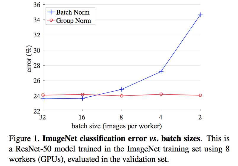
- behaves stably over different batch sizes
- approach BN’s accuracy
论点
- BN
- requires sufficiently large batch size (e.g. 32)
- Mask R-CNN frameworks use a batch size of 1 or 2 images because of higher resolution, where BN is “frozen” by transforming to a linear layer
- synchronized BN 、BR
- LN & IN
- effective for training sequential models or generative models
- but have limited success in visual recognition
- GN能转换成LN/IN
- WN
- normalize the filter weights, instead of operating on features
- BN
方法
group
- it is not necessary to think of deep neural network features as unstructured vectors
- 第一层卷积核通常存在一组对称的filter,这样就能捕获到相似特征
- 这些特征对应的channel can be normalized together
- it is not necessary to think of deep neural network features as unstructured vectors
normalization
transform the feature x:$\hat x_i = \frac{1}{\sigma}(x_i-\mu_i)$
the mean and the standard deviation:
the set $S_i$
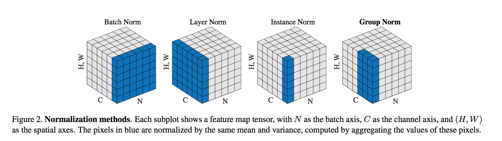
- BN:
- $S_i=\{k|k_C = i_C\}$
- pixels sharing the same channel index are normalized together
- for each channel, BN computes μ and σ along the (N, H, W) axes
- LN
- $S_i=\{k|k_N = i_N\}$
- pixels sharing the same batch index (per sample) are normalized together
- LN computes μ and σ along the (C,H,W) axes for each sample
- IN
- $S_i=\{k|k_N = i_N, k_C=i_C\}$
- pixels sharing the same batch index and the same channel index are normalized together
- LN computes μ and σ along the (H,W) axes for each sample
- GN
- $S_i=\{k|k_N = i_N, [\frac{k_C}{C/G}]=[\frac{i_C}{C/G}]\}$
- computes μ and σ along the (H, W ) axes and along a group of C/G channels
- BN:
linear transform
- to keep representational ability
- per channel
- scale and shift:$y_i = \gamma \hat x_i + \beta$
relation
- to LN
- LN assumes all channels in a layer make “similar contributions”
- which is less valid with the presence of convolutions
- GN improved representational power over LN
- to IN
- IN can only rely on the spatial dimension for computing the mean and variance
- it misses the opportunity of exploiting the channel dependence
- 【QUESTION】BN也没考虑通道间的联系啊,但是计算mean和variance时跨了sample
- to LN
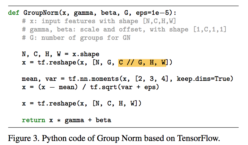
implementation
- reshape
- learnable $\gamma \& \beta$
- computable mean & var
实验
- GN相比于BN,training error更低,但是val error略高于BN
- GN is effective for easing optimization
- loses some regularization ability
- it is possible that GN combined with a suitable regularizer will improve results
- 选取不同的group数,所有的group>1均好于group=1(LN)
- 选取不同的channel数(C/G),所有的channel>1均好于channel=1(IN)
- Object Detection
- frozen:因为higher resolution,batch size通常设置为2/GPU,这时的BN frozen成一个线性层$y=\gamma(x-\mu)/\sigma+beta$,其中的$\mu$和$sigma$是load了pre-trained model中保存的值,并且frozen掉,不再更新
- denote as BN*
- replace BN* with GN during fine-tuning
- use a weight decay of 0 for the γ and β parameters
- GN相比于BN,training error更低,但是val error略高于BN
正则化
综述
正则
正则化是用来解决神经网络过拟合的问题,通过降低模型的复杂性和约束权值,迫使神经网络学习可泛化的特征
- 正则化可以定义为我们为了减少泛化误差而不是减少训练误差而对训练算法所做的任何改变
- 对权重进行约束
- 对目标函数添加额外项(间接约束权值):L1 & L2正则
- 数据增强
- 降低网络复杂度:dropout,stochastic depth
- early stopping
- 我们在对网络进行正则化时不考虑网络的bias:正则表达式只是权值的表达式,不包含bias
- bias比weight具有更少的参数量
- 对bias进行正则化可能引入太多的方差,引入大量的欠拟合
- 正则化可以定义为我们为了减少泛化误差而不是减少训练误差而对训练算法所做的任何改变
L1 & L2:
要惩罚的是神经网络中每个神经元的权重大小
L2关注的是权重的平方和,是要网络中的权重接近0但不等于0,“权重衰减”
L1关注的是权重的绝对值,权重可能被压缩成0,权重更新时每次减去的是一个常量
L1会趋向于产生少量的特征,而其他的特征都是0,而L2会选择更多的特征,这些特征都会接近于0
dropout
- 每个epoch训练的模型都是随机的
- 在test的时候相当于ensemble多个模型
权重共享
数据增强
隐式正则化:其出现的目的不是为了正则化,而正则化的效果是其副产品,包括early stopping,BN,随机梯度下降
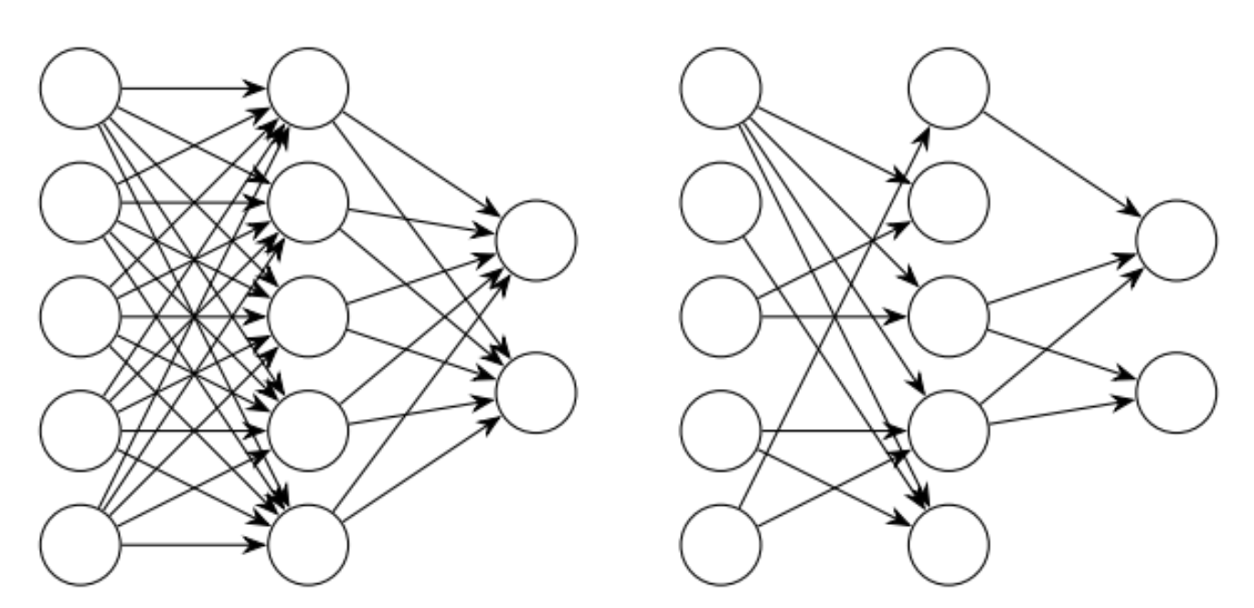
dropout & drop connect([Reference][https://zhuanlan.zhihu.com/p/108024434])
dropout:
- 2012年Hinton提出,在模型训练时以概率p随机让隐层节点的输出变成0,暂时认为这些节点不是网络结构的一部分,但是会把它们的权重保留下来(不更新)。
标准dropout相当于在一层神经元之后再添加一个额外的层,这些神经元在训练期间以一定的概率将值设置为零,并在测试期间将它们乘以p。
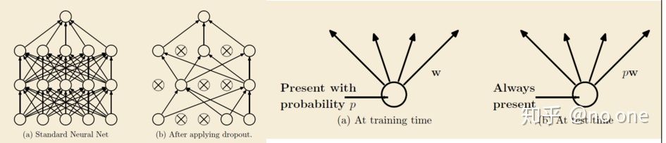
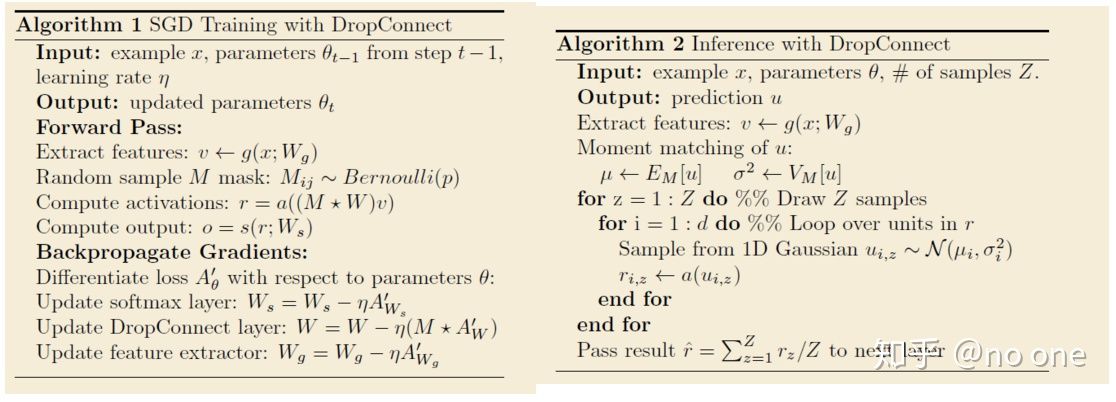
drop connect:
- 不是随机的将隐层节点的输出变成0,而是将节点中的每个与其相连的输入权值以1-p的概率变成0。(一个是输出一个是输入)
- 训练阶段,对每个example/mini-batch, 每个epoch都随机sample一个mask矩阵
Dropconnect在测试期间采用了与标准dropout不同的方法。作者提出了dropconnect在每个神经元处的高斯近似,然后从这个高斯函数中抽取一个样本并传递给神经元激活函数。这使得dropconnect在测试时和训练时都是一种随机方法。
伯努利分布:0-1分布
dropout & drop connect 通常只作用于全连接层上:这俩是用来防止过多参数导致过拟合
卷积层参数贼少,所以没必要,
针对卷积通道有spacial dropout:按照channel随机扔
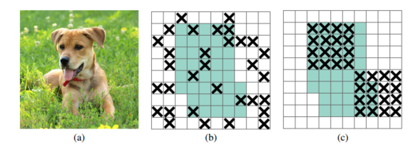
dropblock:是针对卷积层的正则化方法,相比较于dropout的random mute,能够更有效地remove掉部分语义信息,block size=1的时候退化成dropout
papers
[dropout] Improving neural networks by preventing co-adaptation of feature detectors,丢节点
[drop connect] Regularization of neural networks using dropconnect,丢weight path
[Stochastic Depth] Deep Networks with Stochastic Depth,丢layer
[DropBlock] A regularization method for convolutional networks
drop大法一句话汇总
- dropout:各维度完全随机扔
- spacial dropout:按照channel随机扔
- stochastic depth:按照res block随机扔
- dropblock:在feature map上按照spacial块随机扔
- cutout:在input map上按照spacial块随机扔
- dropconnect:扔连接不扔神经元
Deep Networks with Stochastic Depth
动机
- propose a training procedure:stochastic depth,train short and test deep
- for each mini-batch
- randomly drop a subset of layers
- and bypass them with the identity function
- short:reduces training time
- reg:improves the test error
- can increase the network depth
论点
deeper
- expressiveness
- vanishing gradients
- diminishing feature reuse
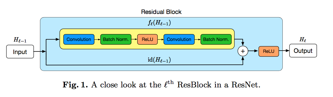
resnet
- skip connection
when输入输出channel数不match:redefine id(·) as a linear projection to reduce the dimensions
dropout
- Dropout reduces the effect known as “co- adaptation” of hidden nodes
- Dropout loses effectiveness when used in combination with Batch Normalization
our approach
- higher diversity
- shorter instead of thinner
- work with Batch Normalization
方法
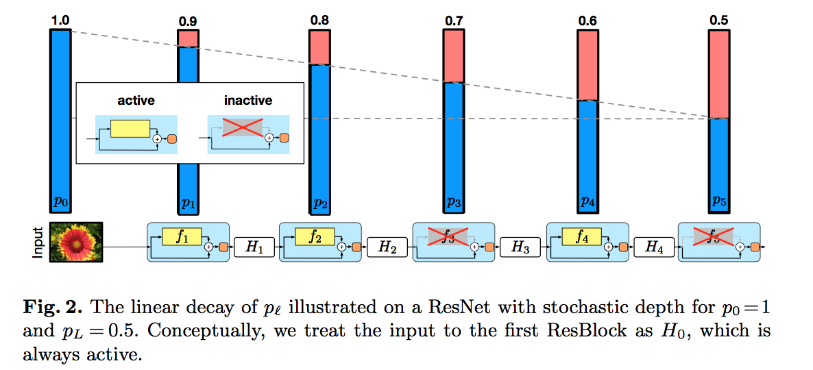
stochastic depth
- randomly dropping entire ResBlocks
- $H_l = ReLU(b_l Res_l(H_{l-1}) + id(H_{l-1}))$
survival probabilities
$p_l = Pr(b_l=1)$
set uniformly / set following a linear decay rule
set $p_0=1, p_L=0.5$:
intuition:the earlier layers extract low-level features that will be used by later layers and should therefore be more reliably present
Expected network depth
- $E(L) \approx 3L/4$
- approximately 25% of training time could be saved
during testing
- all res path are active
- each res path is weighted by its survival probability
- $H_l^{Test} = ReLU(b_l Res_l(H_{l-1}, W_l) + id(H_{l-1}))$
- 跟dropout一样
RetinaNet
- [det] RetinaNet: Focal Loss for Dense Object Detection
- [det+instance seg] RetinaMask: Learning to predict masks improves state-of-the-art single-shot detection for free
- [det+semantic seg] Retina U-Net: Embarrassingly Simple Exploitation of Segmentation Supervision for Medical Object Detection
Focal Loss for Dense Object Detection
动机
- dense prediction(one-stage detector)
- focal loss:address the class imbalance problem
- RetinaNet:design and train a simple dense detector
论点
- accuracy trailed
- two-stage:classifier is applied to a sparse set of candidate
- one-stage:dense sampling of possible object locations
- the extreme foreground-background class imbalance encountered during training of dense detectors is the central cause
- loss
- standard cross entropy loss:down-weights the loss assigned to well-classified examples
- proposed focal loss:focuses training on a sparse set of hard examples
- R-CNN系列two-stage framework
- proposal-driven
- the first stage generates a sparse set of candidate object locations
- the second stage classifies each candidate location as one of the foreground classes or as background
- class imbalance:在stage1大部分背景被filter out了,stage2训练的时候强制固定前背景样本比例,再加上困难样本挖掘OHEM
- faster:reducing input image resolution and the number of proposals
- ever faster:one-stage
- one-stage detectors
- One stage detectors are applied over a regular, dense sampling of object locations, scales, and aspect ratios
- dense:regularly sampling(contrast to selection),基于grid以及anchor以及多尺度
- the training procedure is still dominated by easily classified background examples
- class imbalance:通常引入bootstrapping和hard example mining来优化
- Object Detectors
- Classic:sliding-window+classifier based on HOG,dense predict
- Two-stage:selective Search+classifier based on CNN,shared network RPN
- One-stage:‘anchors’ introduced by RPN,FPN
- loss
- Huber loss:down-weighting the loss of outliers (hard examples)
- focal loss:down-weighting inliers (easy examples)
- accuracy trailed
方法
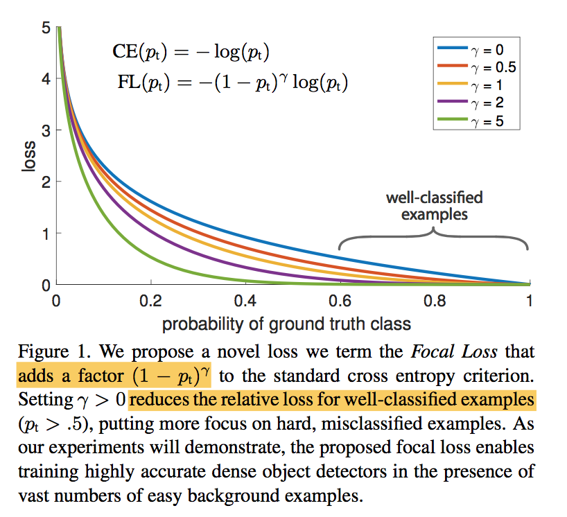
focal loss
- CE:$CE(p_t)=-log(p_t)$
- even examples that are easily classified ($p_t>0.5$) incur a loss with non-trivial magnitude
- summed CE loss over a large number of easy examples can overwhelm the rare class
- WCE:$WCE(p_t)=-\alpha_t log(p_t)$
- balances the importance of positive/negative examples
- does not differentiate between easy/hard examples
FL:$FL(p_t)=-\alpha_t(1-p_t)^\gamma log(p_t)$
- as $\gamma$ increases the modulating factor is likewise increased
- $\gamma=2$ works best in our experiments
two-stage detectors通常不会使用WCE或FL
- cascade stage会过滤掉大部分easy negatives
- 第二阶段训练会做biased minibatch sampling
- Online Hard Example Mining (OHEM)
- construct minibatches using high-loss examples
- scored by loss + nms
- completely discards easy examples
- CE:$CE(p_t)=-log(p_t)$
RetinaNet
- compose:backbone network + two task-specific subnetworks
- backbone:convolutional feature map over the entire input image
- subnet1:object classification
subnet2:bounding box regression
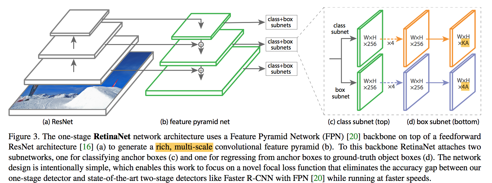
ResNet-FPN backbone
- rich, multi-scale feature pyramid,二阶段的RPN也用了FPN
- each level can be used for detecting objects at a different scale
- P3 - P7:8x - 128x downsamp
- FPN channels:256
anchors
- anchor ratios:{1:2, 1:1, 2:1},长宽比
- anchor scales:{$2^0$, $2^\frac{1}{3}$, $2^\frac{2}{3}$},大小,同一个scale的anchor,面积相同,都是size*size,长宽通过ratio求得
- anchor size per level:[32, 64, 128, 256, 512],基本的正方形anchor的边长
- total anchors per level:A=9
- KA:each anchor is assigned a length K one-hot vector of classification targets
- 4A:and a 4-vector of box regression targets
- anchors are assigned to ground-truth object boxes using an intersection-over-union (IoU) threshold of 0.5
- anchors are assigned background if their IoU is in [0, 0.4)
- anchor is unassigned between [0.4, 0.5), which is ignored during training
- each anchor is assigned to at most one object box
for each anchor
classification targets:one-hot vector
box regression targets:each anchor和其对应的gt box的offset
rpn offset:中心点、宽、高
$$t_x = (x - x_a) / w_a\\
t_y = (y - y_a) / h_a\\t_w = log(w/ w_a)\\
t_h = log(h/ h_a)$$
or omitted if there is no assignment
【QUESTION】所谓的anchor state {-1:ignore, 0:negative, 1:positive} 是针对cls loss来说的,相当于人为丢弃了一部分偏向中立的样本,这对分类效果有提升吗??
classification subnet
for each spatial position,for each anchor,predict one among K classes,one-hot
input:C channels feature map from FPN
structure:four 3x3 conv + ReLU,each with C filters
head:3x3 conv + sigmoid,with KA filters
share across levels
not share with box regression subnet
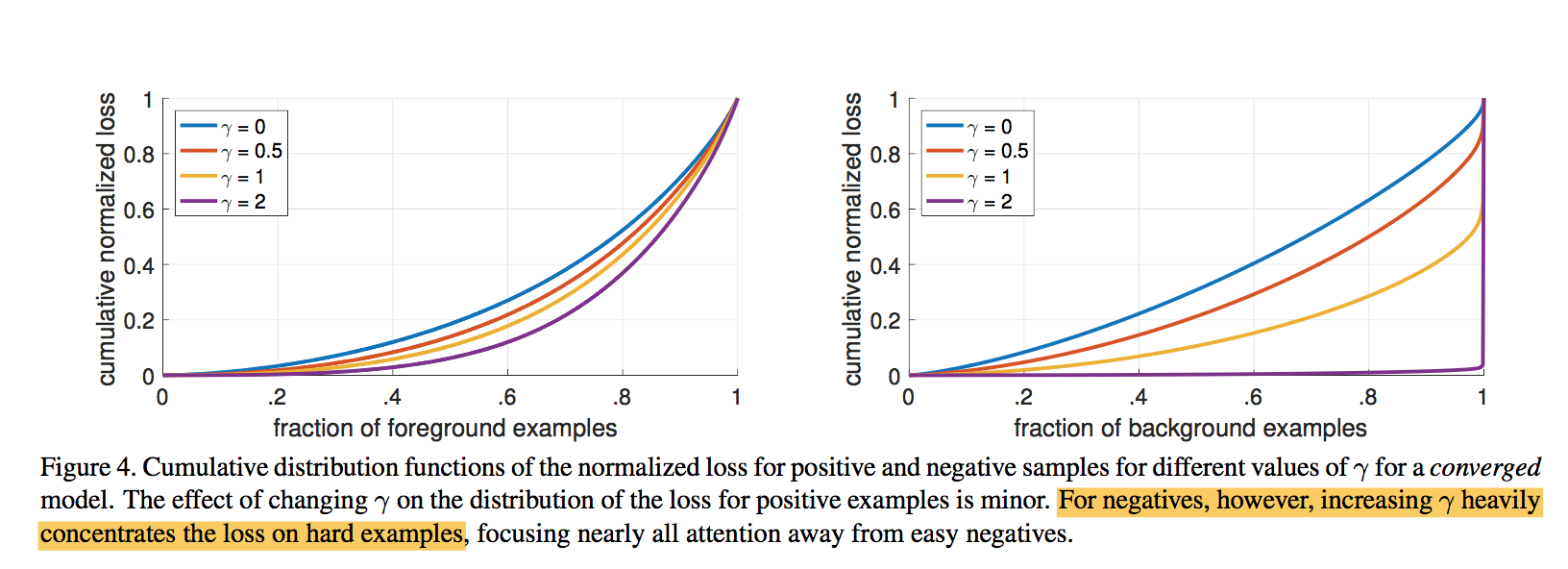
focal loss:
- sum over all ~100k anchors
  * and normalized by the number of anchors assigned to a ground-truth box
  * 因为是sum,所以要normailize,norm项用的是number of assigned anchors(这是包括了前背景?)
  * vast majority of anchors are **easy negatives** and receive negligible loss values under the focal loss(确实包含背景框)
  * $\alpha$:In general $alpha$ should be decreased slightly as $\gamma$ is increased
strong effect on negatives:FL can effectively discount the effect of easy negatives, focusing all attention on the hard negative examples
box regression subnet
- class-agnostic bounding box regressor
- sum over all ~100k anchors
- same structure:four 3x3 conv + ReLU,each with C filters
  * head:4A linear outputs
  * L1 loss
inference
keep top 1k predictions per FPN level
* all levels are merged and non-maximum suppression with a threshold of 0.5train
- initialization:
- cls head bias initialization,encourage more foreground prediction at the start of training
- prevents the large number of background anchors from generating a large, destabilizing loss
- initialization:
network design
anchors
      * one-stage detecors use fixed sampling grid to generate position
      * use multiple ‘anchors’ at each spatial position to cover boxes of various scales and aspect ratios
      * beyond 6-9 anchors did not shown further gains in AP
  * speed/accuracy trade-off
      * outperforms all previous methods
      * bigger resolution bigger AP
      * Retina-101-600与ResNet101-FRCNN的AP持平,但是比他快
gradient:
- 梯度有界
the derivative is small as soon as $x_t > 0$
<img src="RetinaNet/gradient.png" width="70%;" />
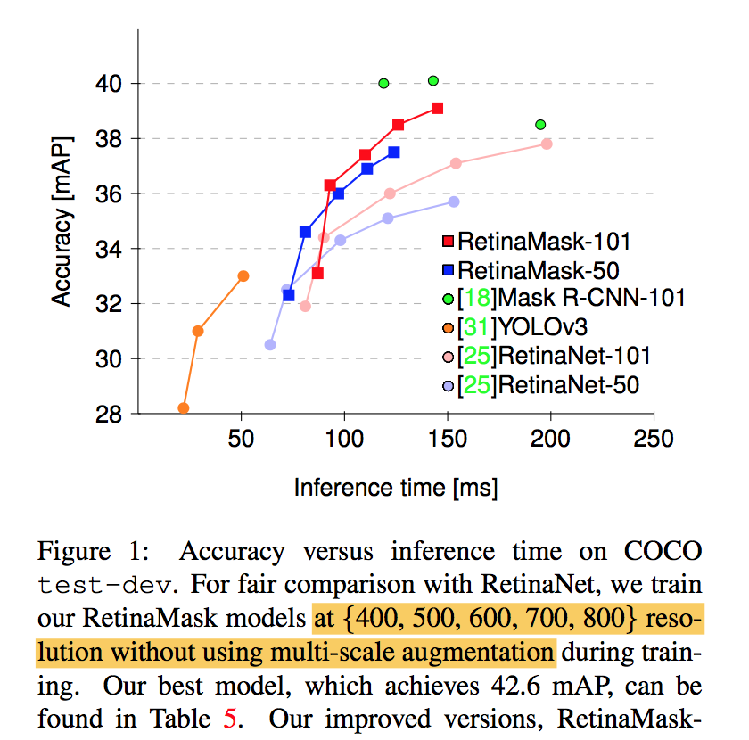
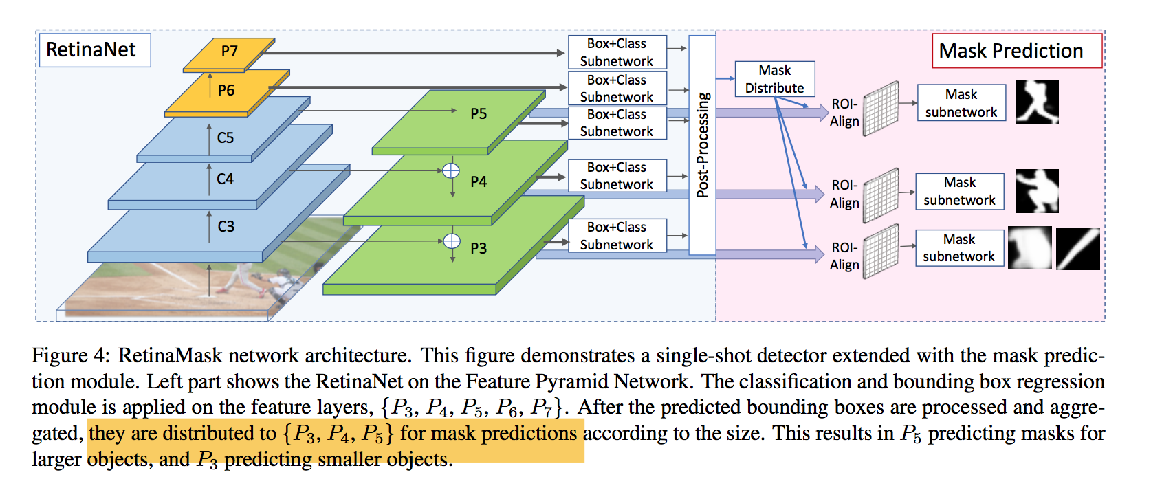
RetinaMask: Learning to predict masks improves state-of-the-art single-shot detection for free
动机
- improve single-shot detectors to the same level as current two-stage techniques
- improve on RetinaNet
- integrating instance mask prediction
- adaptive loss
- additional hard examples
- Group Normalization
same computational cost as the original RetinaNet but more accurate:同样的参数量级比orgin RetinaNet准,整体的参数量级大于yolov3,acc快要接近二阶段的mask RCNN了
论点
- part of improvements of two-stage detectors is due to architectures like Mask R-CNN that involves multiple prediction heads
- additional segmentation task had only been added to two-stage detectors in the past
- two-stage detectors have the cost of resampling(ROI-Align) issue:RPN之后要特征对齐
- add addtional heads in training keeps the structure of the detector at test time unchanged
- potential improvement directions
- data:OHEM
- context:FPN
- additional task:segmentation branch
- this paper’s contribution
- add a mask prediction branch
- propose a new self-adjusting loss function
- include more of positive samples—>those with low overlap
方法
best matching policy
- speical case:outlier gt box,跟所有的anchor iou都不大于0.5,永远不会被当作正样本
- use best matching anchor with any nonzero overlap to replace the threshold
self-adjusting Smooth L1 loss
bbox regression
smooth L1:
- L1 loss is used beyond $\beta$ to avoid over-penalizing outliers
the choice of control point is heuristic and is usually done by hyper parameter search
self-adjusting control point
running mean & variance
minibatch update:m=0.9
control point:$[0, \hat \beta]$ clip to avoid unstable
mask module
detection predictions are treated as mask proposals
extract the top N scored predictions
distribute the mask proposals to sample features from the appropriate layers
- $k_0=4$,如果size小于224*224,proposal会被分配给P3,如果大于448*448,proposal会被分配给P5
- using more feature layers shows no performance boost
architecture
- r50&r101 back:freezing all of the Batch Nor- malization layers
- fpn feature channel:256
- classification branch
- 4 conv layers:conv3x3+relu,channel256
- head:conv3x3+sigmoid,channel n_anchors*n_classes
- regression branch
- 4 conv layers:conv3x3+relu,channel256
- head:conv3x3,channel n_anchors*4
- aggregate the boxes to the FPN layers
- ROI-Align yielding 14x14 resolution features
mask head
- 4 conv layers:conv3x3
- a single transposed convolutional layer:convtranspose2d 2x2,to 28*28 resolution
- prediction head:conv1x1
training
- min side & max side:800&1333
- limited GPU:reduce the batch size,increasing the number of training iterations and reducing the learning rate accordingly
- positive/ignore/negative:0.5,0.4
focal loss for classification
gaussian initialization
$\alpha=0.25, \lambda=2.0$
$FL=-\alpha_t(1-p_t)^\lambda log(p_t)$
gamma项控制的是简单样本的衰减速度,alpha项控制的是正负样本比例,可以默认值下正样本的权重是0.25,负样本的权重是0.75,和想象中的给正样本更多权重不一样,因为alpha和gamma是耦合起来作用的,(可能检测场景下困难的负样本相比于正样本更少?背景就是比前景好学?不确定不确定。。。)
- self-adjusting L1 loss for box regression
- limit running params:[0, 0.11]
- mask loss
- top-100 predicted boxes + ground truth boxes
inference
- box confidence threshold 0.05
- nms threshold 0.4
- use top-50 boxes for mask prediction
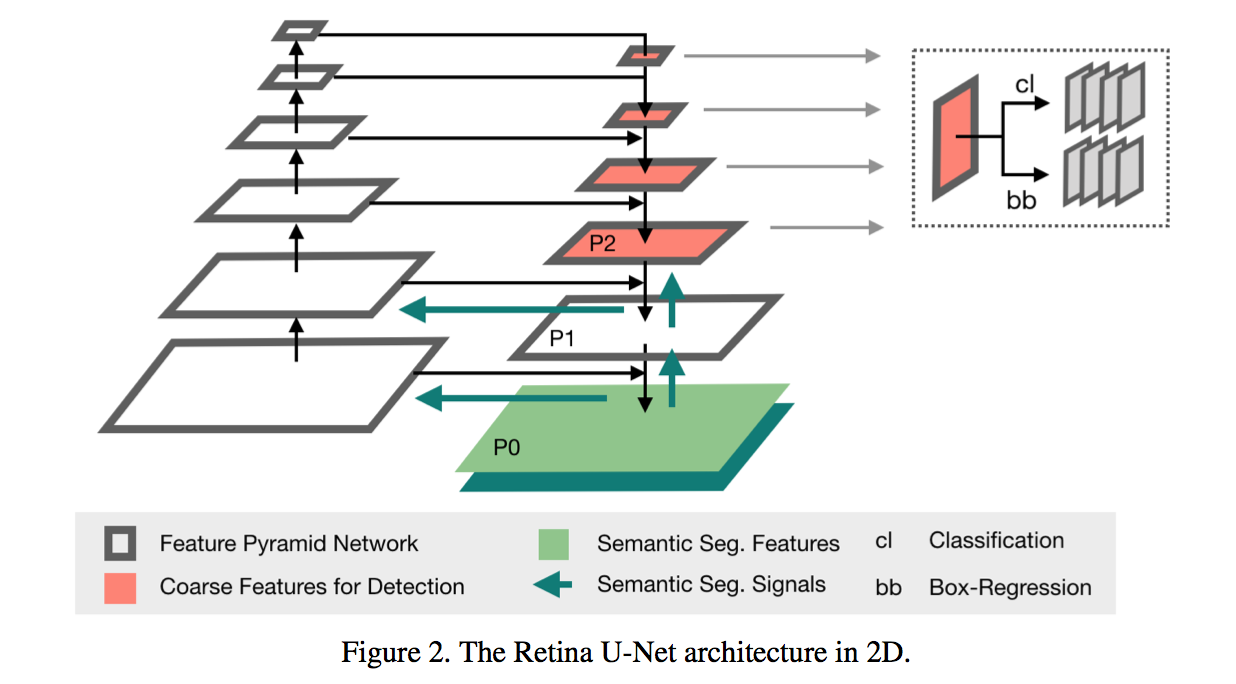
Retina U-Net: Embarrassingly Simple Exploitation of Segmentation Supervision for Medical Object Detection
动机
- localization
- pixel-level predict
- ad-hoc heuristics when mapping back to object-level scores
- semantic segmentation
- auxiliary task
- overall one-stage
- leveraging available supervision signals
- localization
论点
- monitoring pixel-wise predictions are clinically required
- medical annotations is commonly performed in pixel- wise
- full semantic supervision
- fully exploiting the available semantic segmentation signal results in significant performance gains
- one-stage
- explicit scale variance enforced by the resampling operation in two-stage detectors is not helpful in the medical domain
- two-stage methods
- predict proposal-based segmentations
- mask loss is only evaluated on cropped proposal:no context gradients
- ROI-Align:not suggested in medical image
- depends on the results of region proposal:serial vs parallel
- gradients of the mask loss do not flow through the entire model
方法
model
- back:
- ResNet50
- fpn:
- shift p3-p6 to p2-p5
- change sigmoid to softmax
- 3d head channels:64
- anchor size:$\{P_2: 4^2, P_3: 8^2,, P_4: 16^2,, P_5: 32^2\}$
- 3d z-scale:{1,2,4,8},考虑到z方向的low resolution
- segmentation supervision
- p0 & p1
- with skip connections
- without detection heads
- segmentation loss calculates on p0 logits
- dice + ce
h
- back:
weighted box clustering
patch crop
tiling strategies & model ensembling causes multi predictions per location
nms选了一类中score最大的box,然后抑制所有与它同类的IoU大于一定阈值的box
weighted box作用于这一类所有的box,计算一个融合的结果
- coordinates confidence:$o_c = \frac{\sum c_i s_i w_i}{\sum s_i w_i}$
score confidence:$o_s = \frac{\sum s_i w_i}{\sum w_i + n_{missing * \overline w}}$
$w_i$:$w=f a p$
- overlap factor f:与highest scoring box的overlap
- area factor a:higher weights to larger boxes,经验
- patch center factor p:相对于patch center的正态分布
- score confidence的分母上有一个down-weight项$n_{missing}$:基于prior knowledge预期prediction的总数得到
论文给的例子让我感觉好比nms的点
- 一个cluster里面一类最终就留下一个框:解决nms一类大框包小框的情况
- 这个location上prediction明显少于prior knowledge的类别confidence会被显著拉低:解决一个位置出现大概率假阳框的情况
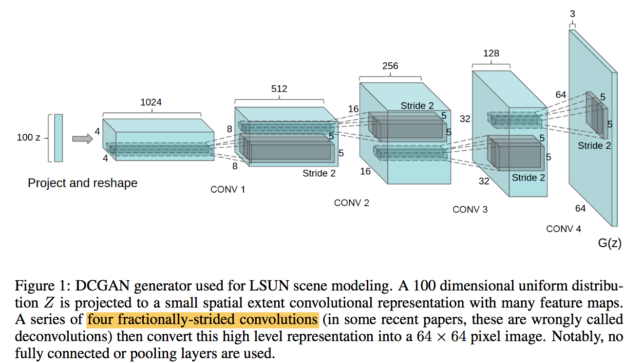
DCGAN
UNSUPERVISED REPRESENTATION LEARNING WITH DEEP CONVOLUTIONAL GENERATIVE ADVERSARIAL NETWORKS
动机
- unsupervised learning
- learns a hierarchy of representations from object parts to scenes
- used for novel tasks
论点
- GAN
- Learning reusable feature representations from large unlabeled datasets
- generator and discriminator networks can be later used as feature extractors for supervised tasks
- unstable to train
- we
- propose a set of constraints on the architectural topology making it stable to train
- use the trained discriminators for image classification tasks
- visualize the filters
- show that the generators have interesting vector arithmetic properties
- unsupervised representation learning
- clustering, hierarchical clustering
- auto-encoders learn good feature representations
- generative image models
- samples often suffer from being blurry, being noisy and incomprehensible
- further use for supervised tasks
- GAN
方法
architecture
- all convolutional net:没有池化,用stride conv
- eliminating fully connected layers:
- generator:输入是一个向量,reshape以后接的全是卷积层
- discriminator:最后一层卷积出来直接flatten
- Batch Normalization
- generator输出层 & discriminator输入层不加
- resulted in sample oscillation and model instability
ReLU
- generator输出层用Tanh
- discriminator用leakyReLU
train
- image preprocess:rescale to [-1,1]
- LeakyReLU(0.2)
- lr:2e-4
- momentum term $\beta 1$:0.5, default 0.9
实验
- evaluate
- apply them as a feature extractor on supervised datasets
- evaluate the performance of linear models on top of these features
- model
- use the discriminator’s convolutional features from all layers
- maxpooling to 4x4 grids
- flattened and concatenated to form a 28672 dimensional vector
- regularized linear L2-SVM
- 相比之下:the discriminator has many less feature maps, but larger total feature vector size
- visualizing
- walking in the latent space
- 在vector Z上差值,生成图像可以观察到smooth transitions
- visualize the discriminator feature
- 特征图可视化,能观察到床结构
- manipulate the generator representation
- generator learns specific object representations for major scene components
- use logistic regression to find feature maps related with window, drop the spatial locations on feature-maps
- most result forgets to draw windows in the bedrooms, replacing them with other objects
- walking in the latent space
- vector arithmetic
- averaging the Z vector for three examplars
- semantically obeyed the arithmetic
- evaluate
densenet
动机
- embrace shorter connections
- the feature-maps of all preceding layers are used as inputs
- advantages
- alleviate vanishing-gradient
- encourage feature reuse
- reduce the number of parameters
论点
- Dense
- each layer obtains additional inputs from all preceding lay- ers and passes on its own feature-maps to all subsequent layers
- feature reuse
- combine features by concatenating:the summation in ResNet may impede the information flow in the network
- information preservation
- id shortcut/additive identity transformations
fewer params
- DenseNet layers are very narrow
- add only a small set of feature-maps to the “collective knowledge”
gradients flow
- each layer has direct access to the gradients from the loss function
- have regularizing effect
- Dense
方法
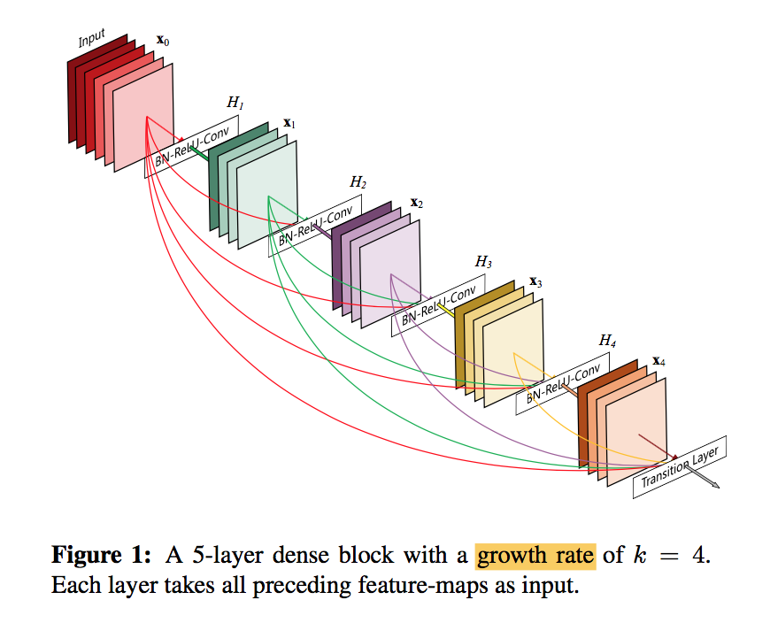
architecture
- dense blocks
- concat
- BN-ReLU-3x3 conv
- $x_l = H_l([x_0, x_1, …, x_{l-1}])$
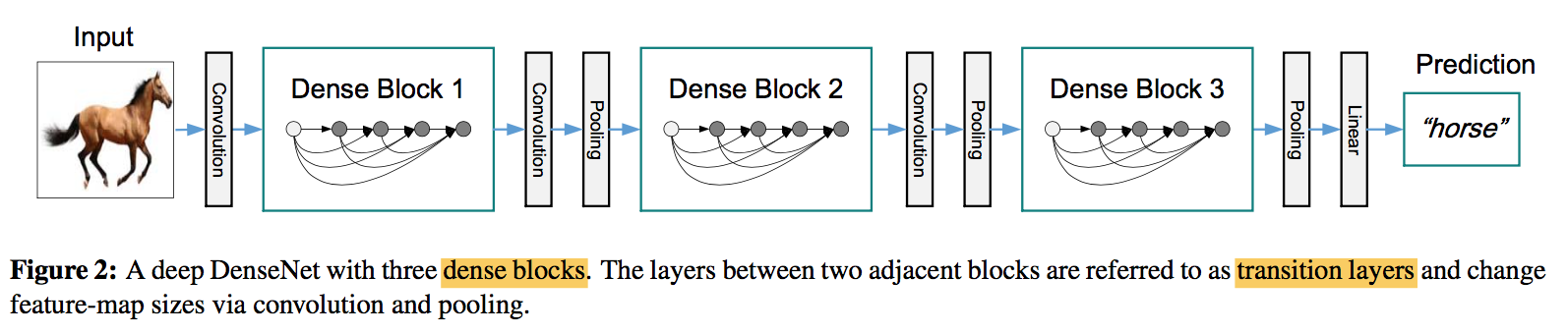
- transition layers
- change the size of feature-maps
- BN-1x1 conv-2x2 avg pooling
growth rate k
- $H_l$ produces feature- maps
- narrow:e.g., k = 12
- One can view the feature-maps as the global state of the network
- The growth rate regulates how much new information each layer contributes to the global state
bottleneck —- DenseNet-B
- in dense block stage
- 1x1 conv reduce dimension first
- number of channels:4k
compression —- DenseNet-C
- in transition stage
- reduce the number of feature-maps
- number of channels:$\theta k$
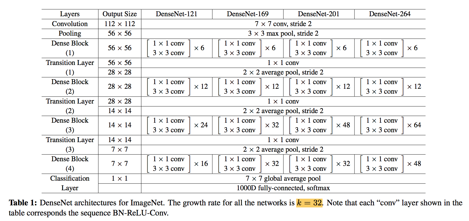
structure configurations
- 1st conv channels:第一层卷积通道数
- number of dense blocks
- L:dense block里面的layer数
- k:growth rate
- B:bottleneck 4k
- C:compression 0.5k
- dense blocks
讨论
concat replace sum:
- seemingly small modification lead to substantially different behaviors of the two network architectures
- feature reuse:feature can be accessed anywhere
- parameter efficient:同样参数量,test acc更高,同样acc,参数量更少
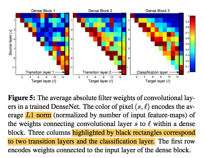
deep supervision:classifiers attached to every hidden layer
weight assign
- All layers spread their weights over multi inputs (include transition layers)
- least weight are assigned to the transition layer, indicating that transition layers contain many redundant features, thus can be compressed
- overall there seems to be concentration towards final feature-maps, suggesting that more high-level features are produced late in the network
GANomaly
GANomaly: Semi-Supervised Anomaly Detection via Adversarial Training
动机
- Anomaly detection
- highly biased towards one class (normal)
- insufficient sample size of the other class (abnormal)
- semi-supervised learning
- detecting the unknown/unseen anomaly case
- trained on normal samples
- tested on normal and abnormal samples
- encoder-decoder-encoder
- minimizing the distance between the images
- and the latent vectors
- a larger distance metric
- Anomaly detection
论点
- supervised approaches heavily depend on large, labeled datasets
- Generative Adversarial Networks (GAN) have emerged as a leading methodology across both unsupervised and semi-supervised problems
- reconstruction-based anomaly techniques
- Overall prior work strongly supports the hypothesis that the use of autoencoders and GAN
方法
- GAN
- unsupervised
- to generate realistic images
- compete
- generator tries to generate an image, decoder- alike network, map input to latent space
- discriminator decides whether the generated image is a real or a fake, classical classification architecture, reading an input image, and determining its validity
Adversarial Auto-Encoders (AAE)
- encoder + decoder
- reconstruction: maps the input to latent space and remaps back to input data space
- train autoencoders with adversarial setting
inverse mapping
- with the additional use of an encoder, a vanilla GAN network is capable of learning inverse mapping
model
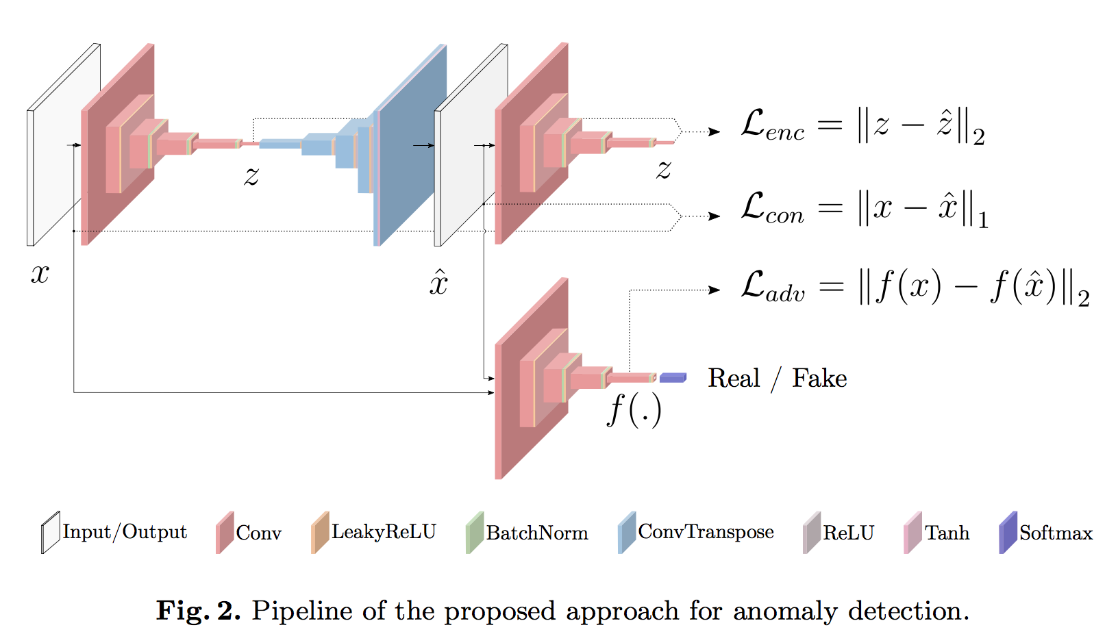
- learns both the normal data distribution and minimizes the output anomaly score
- two encoder, one decoder, a discriminator
- encoder
- convolutional layers followed by batch-norm and leaky ReLU() activation
- compress to a vector z
- decoder
- convolutional transpose layers, ReLU() activation and batch-norm
- a tanh layer at the end
- 2nd encoder
- with the same architectural
- but different parametrization
- discriminator
- DCGAN discriminator
- Adversarial Loss
- 不是基于GAN的traditional 0/1 ouput
- 而是选了一个中间层,计算real/fake(reconstructed)的L2 distance
- Contextual Loss
- L1 yields less blurry results than L2
- 计算输入图像和重建图像的L1 distance
- Encoder Loss
- an additional encoder loss to minimize the distance of the bottleneck features
- 计算两个高维向量的L2 distance
- 在测试的时候用它来scoring the abnormality
- GAN
resnets
overview
papers
[resnet] ResNet: Deep Residual Learning for Image Recognition
[resnext] ResNext: Aggregated Residual Transformations for Deep Neural Networks
[resnest] ResNeSt: Split-Attention Networks
[revisiting resnets] Revisiting ResNets: Improved Training and Scaling Strategies
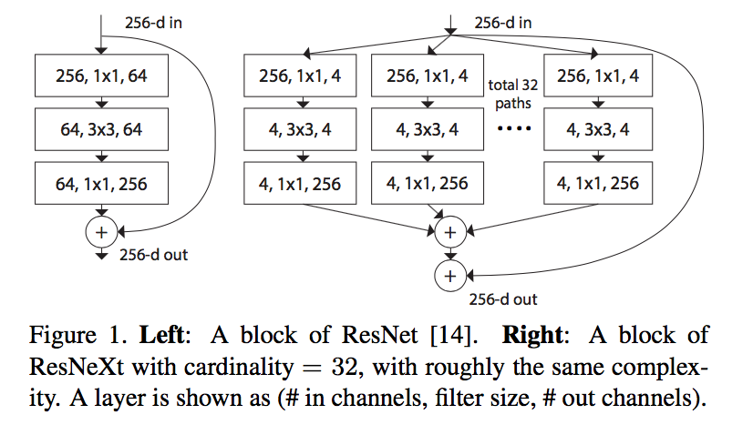
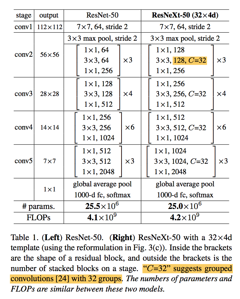
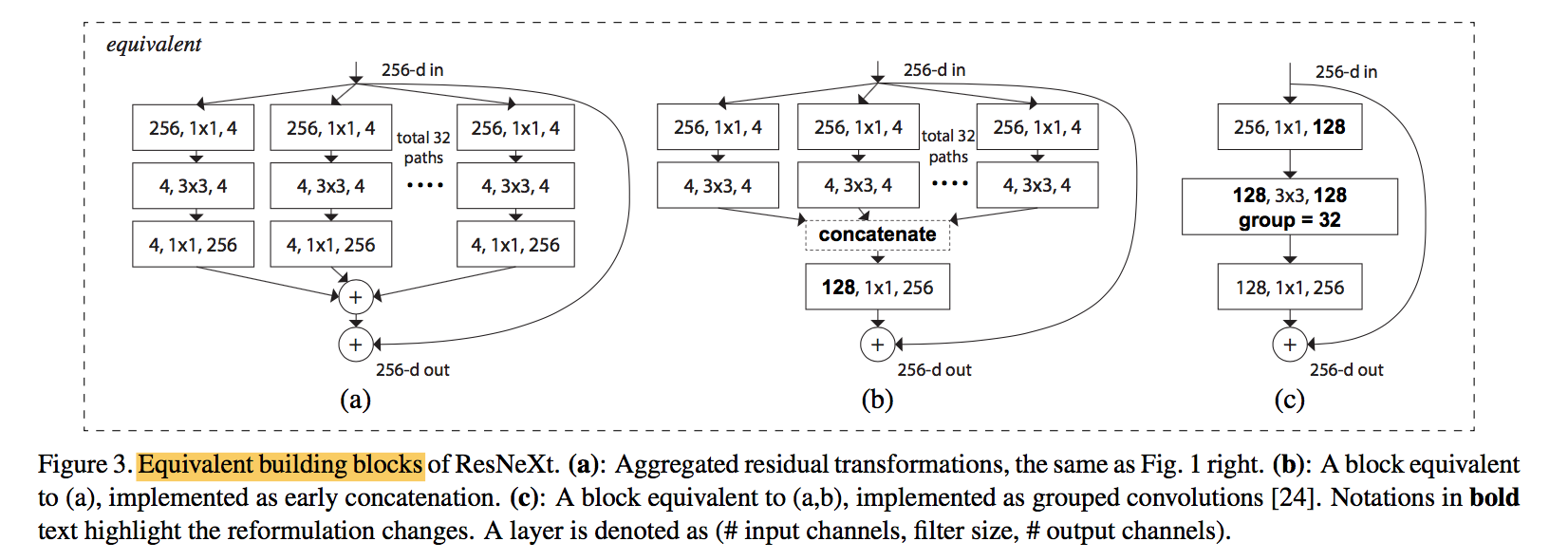
ResNext: Aggregated Residual Transformations for Deep Neural Networks
动机
- new network architecture
- new building blocks with the same topology
- propose cardinality
- increasing cardinality is able to improve classification accuracy
- is more effective than going deeper or wider
- classification task
论点
VGG & ResNets:
- stacking building blocks of the same topology
- deeper
- reduces the free choices of hyper-parameters
Inception models
- split-transform-merge strategy
- split:1x1conv spliting into a few lower-dimensional embeddings
- transform:a set of specialized filters
merge:concat
approach the representational power of large and dense layers, but at a considerably lower computational complexity
- modules are customized stage-by-stage
our architecture
- adopts VGG/ResNets’ repeating layers
- adopts Inception‘s split-transform-merge strategy
- aggregated by summation
cardinality:the size of the set of transformations(split path数)
- 多了1x1 conv的计算量
- 少了3x3 conv的计算量
要素
- Multi-branch convolutional blocks
- Grouped convolutions:通道对齐,稀疏连接
- Compressing convolutional networks
- Ensembling
方法
architecture
- a template module
- if producing spatial maps of the same size, the blocks share the same hyper-parameters (width and filter sizes)
when the spatial map is downsampled by a factor of 2, the width of the blocks is multiplied by a factor of 2
grouped convolutions:第一个1x1和3x3conv的width要根据C进行split
equivalent blocks
- BN after each conv
- ReLU after each BN except the last of block
- ReLU after add
r
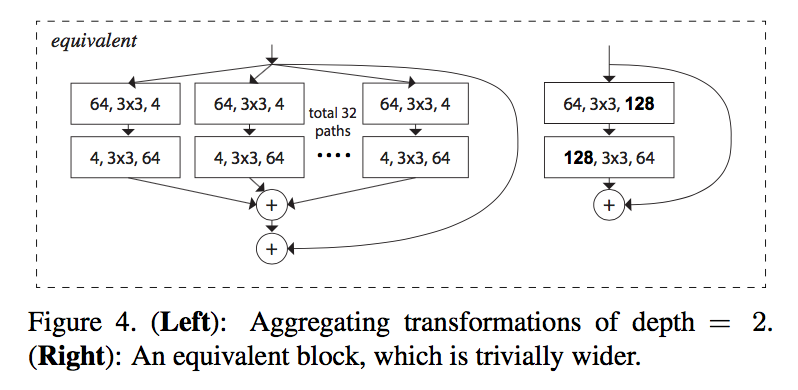
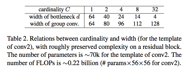
Model Capacity
improve accuracy when maintaining the model complexity and number of parameters
adjust the width of bottleneck, the according C to maintain capacity:C=1的时候退化成ResNet block
ResNeSt: Split-Attention Networks
动机
- propose a modular Split-Attention block
- enables attention across feature-map groups
- preserve the overall ResNet structure for downstream applications such as object detection and semantic segmentation
- prove improvement on detection & segmentation tasks
论点
- ResNet
- simple and modular design
- limited receptive-field size and lack of cross-channel interaction
- image classification networks have focused more on group or depth-wise convolution
- do not transfer well to other tasks
- isolated representations cannot capture cross-channel relationships
- a versatile backbone
- improving performance across multiple tasks at the same time
- a network with cross-channel representations is desirable
- a Split-Attention block
- divides the feature-map into several groups (along the channel dimension)
- finer-grained subgroups or splits
- weighted combination
- featuremap attention mechanism:NiN’s 1x1 conv
- Multi-path:GoogleNet
- channel-attention mechanism:SE-Net
结构上,全局上看,模仿ResNext,引入cardinality和group conv,局部上看,每个group内部继续分组,然后模仿SK-Net,融合多个分支的split-attention,大group之间concat,而不是ResNext的add,再经1x1 conv调整维度,add id path

- ResNet
方法
Split-Attention block
enables feature-map attention across different feature-map groups
within a block:controlled by cardinality
within a cardinal group:introduce a new radix hyperparameter R indicating the number of splits
split-attention
- 多个in-group branch的input输入进来
- fusion:先做element-wise summation
- channel-wise global contextual information:做global average pooling
- 降维:Dense-BN-ReLU
- 各分支Dense(the attention weight function):学习各自的重要性权重
- channel-wise soft attention:对全部的dense做softmax
- 加权:原始的各分支input与加权的dense做乘法
- 和:加权的各分支add
r=1:退化成SE-blockaverage pooling

shortcut connection
- for blocks with a strided convolution or combined convolution-with-pooling can be applied to the id
concat
average pooling downsampling
- for dense prediction tasks:it becomes essential to preserve spatial information
- former work tend to use strided 3x3 conv
- we use an average pooling layer with 3x3 kernel
- 2x2 average pooling applied to strided shortcut connection before 1x1 conv
Revisiting ResNets: Improved Training and Scaling Strategies
动机
disentangle the three aspects
- model architecture
- training methodology
- scaling strategies
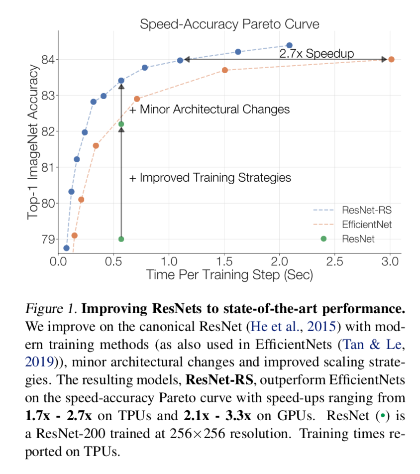
improve ResNets to SOTA
- design a family of ResNet architectures, ResNet-RS
- use improved training and scaling strategies
- and combine minor architecture changes
- 在ImageNet上打败efficientNet
在半监督上打败efficientNet-noisystudent
论点
- ImageNet上榜大法
- Architecture
- 人工系列:AlexNet,VGG,ResNet,Inception,ResNeXt
- NAS系列:NasNet-A,AmoebaNet-A,EfficientNet
- Training and Regularization Methods
- regularization methods
- dropout,label smoothing,stochastic depth,dropblock,data augmentation
- significantly improve generalization when training more epochs
- training
- learning rate schedules
- regularization methods
- Scaling Strategies
- model dimension:width,depth,resolution
- efficientNet提出的均衡增长,在本文中shows sub-optimal for both resnet and efficientNet
- Additional Training Data
- pretraining on larger dataset
- semi-supervised
- Architecture
- the performance of a vision model
- architecture:most research focus on
- training methods and scaling strategy:less publicized but critical
- unfair:使用modern training method的新架构与使用dated methods的老网络直接对比
- we focus on the impact of training methods and scaling strategies
- training methods:
- We survey the modern training and regularization techniques
- 发现引入其他正则方法的时候降低一点weight decay有好处
- scaling strategies:
- We offer new perspectives and practical advice on scaling
- 可能出现过拟合的时候就加depth,否则先加宽
- resolution慢点增长,more slowly than prior works
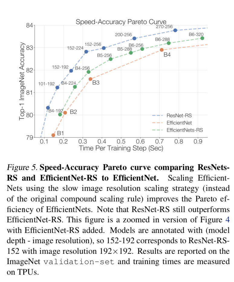
- 从acc图可以看到:我们的scaling strategies与网络结构的lightweight change正交,是additive的
- training methods:
- re-scaled ResNets, ResNet-RS
- 仅improve training & scaling strategy就能大幅度涨点
- combine minor architectural changes进一步涨点
- ImageNet上榜大法
方法
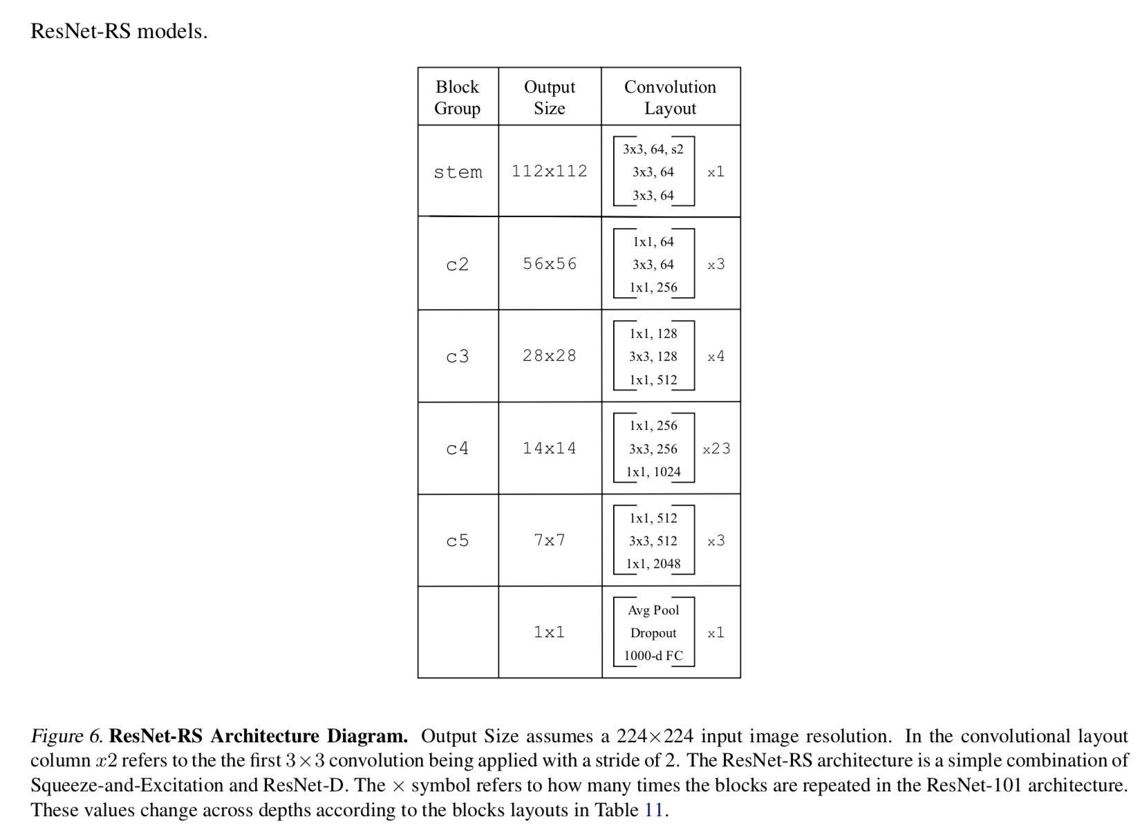
architecture
- use ResNet with two widely used architecture changes
- ResNet-D
- stem的7x7conv换成3个3x3conv
- stem的maxpooling去掉,每个stage的首个3x3conv负责stride2
- residual path上前两个卷积的stride互换(在3x3上下采样)
- id path上的1x1 s2conv替换成2x2 s2的avg pooling+1x1conv
SE in bottleneck
- use se-ratio of 0.25
training methods
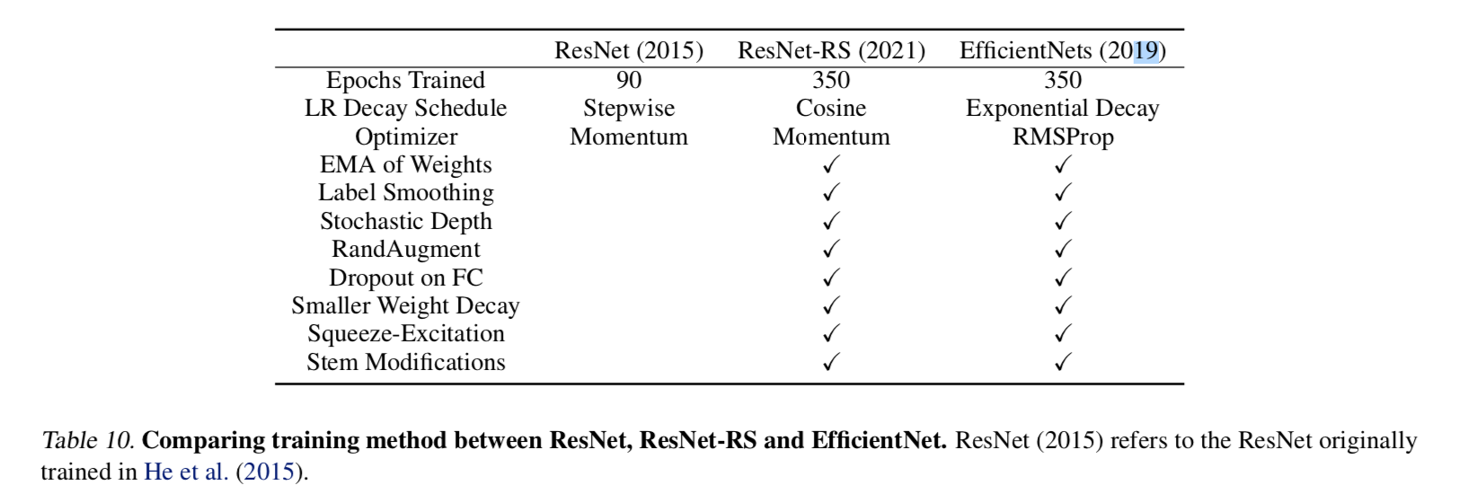
- match the efficientNet setup
- train for 350 epochs
- use cosine learning rate instead of exponential decay
- RandAugment instead of AutoAugment
- use Momentum optimizer instead of RMSProp
- regularization
- weight decay
- label smoothing
- dropout
- stochastic depth
data augmentation
- we use RandAugment
- EfficientNet use AutoAugment which slightly outperforms RandAugment
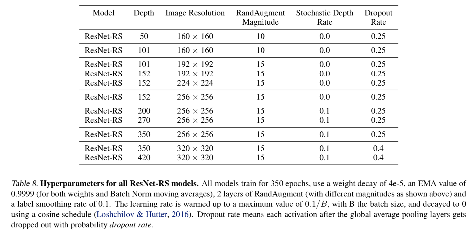
hyper:
- droprate
- increase the regularization as the model size increase to limit overfitting
- label smoothing = 0.1
- weight decay = 4e-5
- match the efficientNet setup
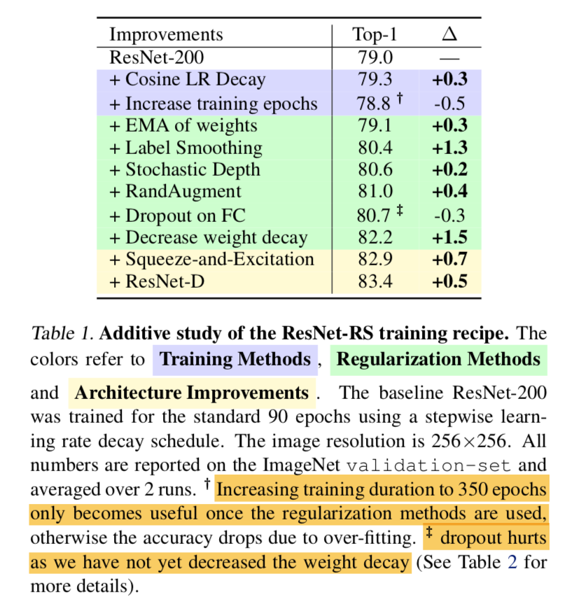
improved training methods
additive study
- 总体上看都是additive的
- increase training epochs在添加regularization methods的前提下才不hurt,否则会overfitting
dropout在不降低weight decay的情况下会hurt
weight decay
- 少量/没有regularization methods的情况下:大weight decay防止过拟合,1e-4
- 多/强regularization methods的情况下:适当减小weight decay能涨点,4e-5
improved scaling strategies
search space
- width multiplier:[0.25, 0.5, 1.0, 1.5, 2.0]
- depth:[26, 50, 101, 200, 300, 350, 400]
- resolution:[128, 160, 224, 320, 448]
- increase regularization as model size increase
- observe 10/100/350 epoch regime
we found that the best scaling strategies depends on training regime
strategy1:scale depth
- Depth scaling outperforms width scaling for longer epoch regimes
- width scaling is preferable for shorter epoch regimes
- scaling width可能会引起overfitting,有时候会hurt performance
- depth scaling引入的参数量也比width小
strategy2:slow resolution scaling
- efficientNets/resNeSt lead to very large images
our experiments:大可不必
实验
Receptive Field
综述
感受野
除了卷积和池化,其他层并不影响感受野大小
感受野与卷积核尺寸kernel_size和步长stride有关
递归计算:
其中$cur_RF$是当前层(start from 1),$kernel_size$、$stride$是当前层参数,$N_RF$是上一层的感受野。
Understanding the Effective Receptive Field in Deep Convolutional Neural Networks
动机
effective receptive field
the effect of nonlinear activations, dropout, sub-sampling and skip connections on it
论点
- it is critical for each output pixel to have a big receptive field, such that no important information is left out when making the prediction
- deeper network:increase the receptive field size linearly
- Sub-sampling:increases the receptive field size multiplicatively
- it is easy to see that pixels at the center of a receptive field have a much larger impact on an output:前向传播的时候,中间位置的像素点有更多条path通向output
方法看不懂直接看结论
dropout does not change the Gaussian ERF shape
Subsampling and dilated convolutions turn out to be effective ways to increase receptive field size quickly
Skip-connections make ERFs smaller
ERFs are Gaussian distributed
- uniformly和随机初始化都是perfect Gaus- sian shapes
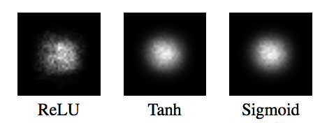
加上非线性激活函数以后是near Gaussian shapes
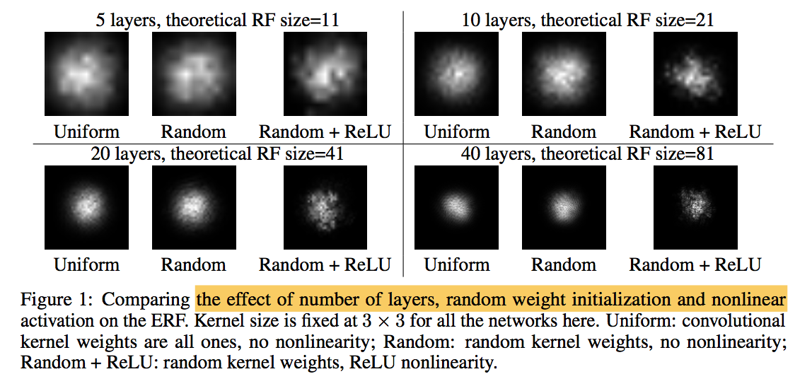
with different nonlinearities
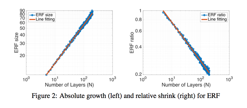
$\sqrt n$ absolute growth and $1/\sqrt n$ relative shrinkage:RF是随着layer线性增长的,ERF在log上0.56的斜率,约等于$\sqrt n$
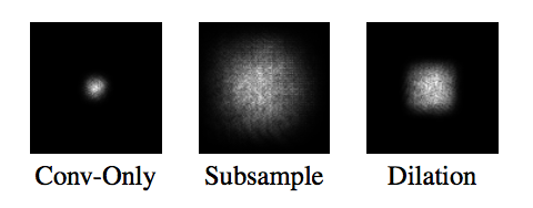
Subsampling & dilated convolution increases receptive field
- The reference baseline is a convnet with 15 dense convolution layers
- Subsampling:replace 3 of the 15 convolutional layers with stride-2 convolution
dilated:replace them with dilated convolution with factor 2,4 and 8,rectangular ERF shape
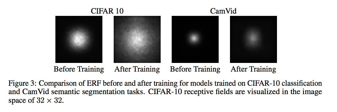
evolves during training
- as the networks learns, the ERF gets bigger, and at the end of training is significantly larger than the initial ERF
- classification
- 32*32 cifar 10
- theoretical receptive field of our network is actually 74 × 74
- segmentation
- CamVid dataset
- the theoretical receptive field of the top convolutional layer units is quite big at 505 × 505
实际的ERF都很小,都没到原图大小
increase the effective receptive field
- New Initialization:
- makes the weights at the center of the convolution kernel to have a smaller scale, and the weights on the outside to be larger
- 30% speed-up of training
- 其他效果不明显
- Architecturalchanges
- sparsely connect each unit to a larger area
- dilated convolution or even not grid-like
- New Initialization:
g
SqueezeNet
SQUEEZENET: ALEXNET-LEVEL ACCURACY WITH 50X FEWER PARAMETERS AND <0.5MB MODEL SIZE
动机
- Smaller CNN
- achieve AlexNet-level accuracy
- model compression
论点
- model compression
- SVD
- sparse matrix
- quantization (to 8 bits or less)
- CNN microarchitecture
- extensively 3x3 filters
- 1x1 filters
- higher level building blocks
- bypass connections
- automated designing approaches
- this paper eschew automated approaches
- propose and evaluate the SqueezeNet architecture with and without model compression
- explore the impact of design choices
- model compression
方法
architectural design strategy
- Replace 3x3 filters with 1x1 filters
- Decrease the number of input channels to 3x3 filters (squeeze)
- Downsample late in the network so that convolution layers have large activation maps:large activation maps (due to delayed downsampling) can lead to higher classification accuracy
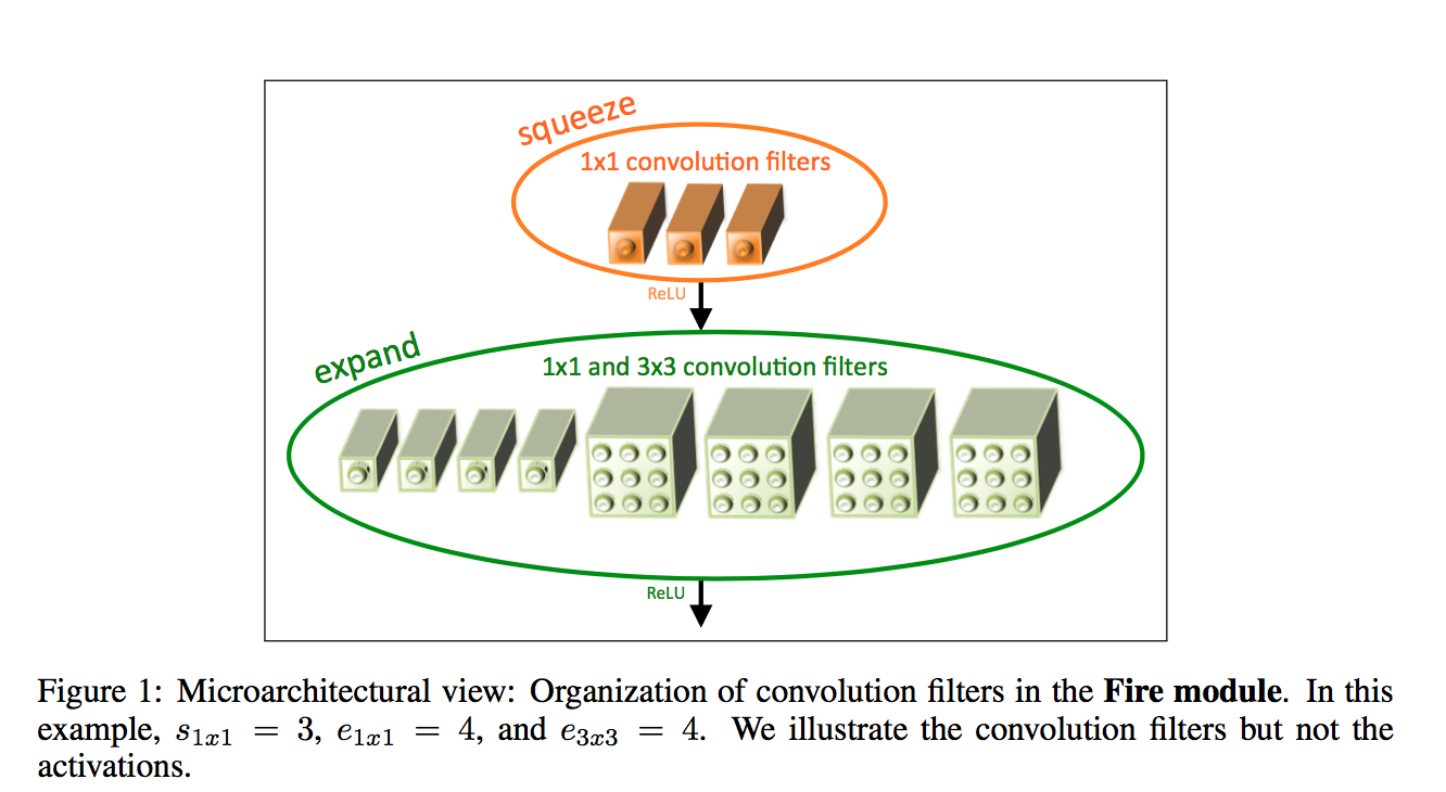
the fire module
- squeeze:1x1 convs
- expand:mix of 1x1 and 3x3 convs, same padding
- relu
concatenate
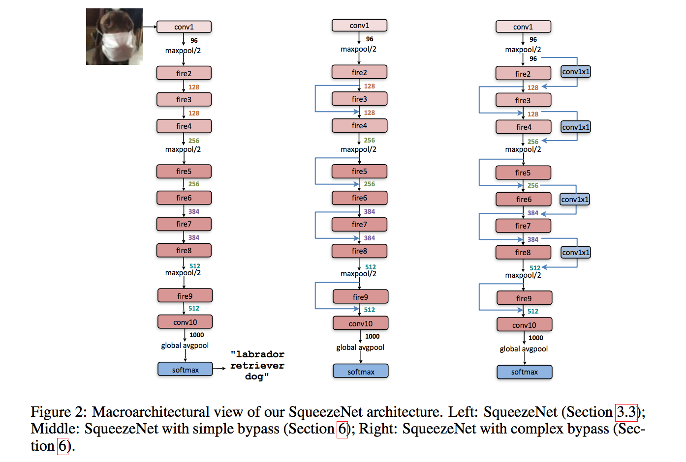
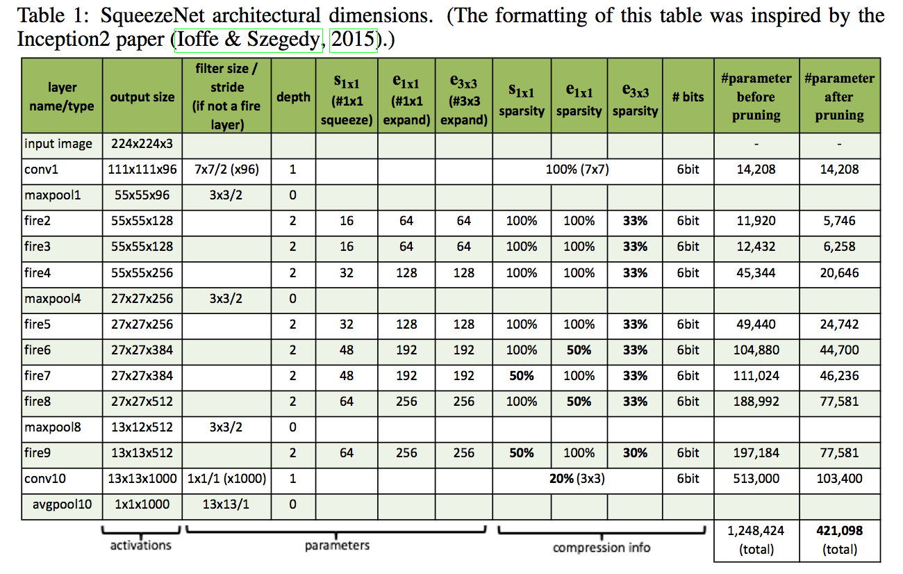
the SqueezeNet
- a standalone convolution layer (conv1)
- followed by 8 Fire modules (fire2-9)
- ending with a final conv layer (conv10)
- stride2 max-pooling after layers conv1, fire4, fire8, and conv10
- dropout with a ratio of 50% is applied after the fire9 module
GAP
understand the impact
each Fire module has three dimensional hyperparameters, to simplify:
- define $base_e$:the number of expand filters in the first Fire module
- for layer i:$e_i=base_e + (incr_e*[\frac{i}{freq}])$
- expand ratio $pct_{3x3}$:the percentage of 3x3 filters in expand layers
- squeeze ratio $SR$:the number of filters in the squeeze layer/the number of filters in the expnad layer
- normal setting:$base_e=128, incre_e=128, pct_{3x3}=0.5, freq=2, SR=0.125$
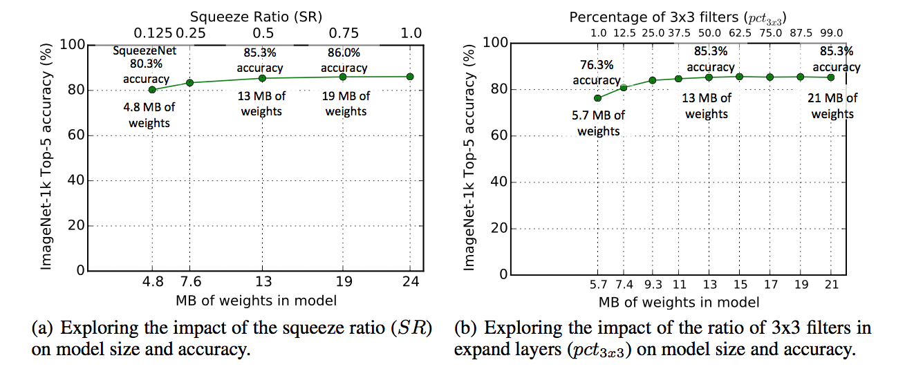
SR
- increasing SR leads to higher accuracy and larger model size
- Accuracy plateaus at 86.0% with SR=0.75
- further increasing provides no improvement
pct
- increasing pct leads to higher accuracy and larger model size
- Accuracy plateaus at 85.6% with pct=50%
- further increasing provides no improvement
bypass
- Vanilla
- simple bypass:when in & out channels have the same dimensions
- complex bypass:includes a 1x1 convolution layer
- alleviate the representational bottleneck introduced by squeeze layers
- both yielded accuracy improvements
- simple bypass enabled higher accuracy