pseudo-3d

发表于 2020-09-02 |

[3d resnet] Learning Spatio-Temporal Features with 3D Residual Networks for Action Recognition：真3d，for comparison，分类

[C3d] Learning Spatiotemporal Features with 3D Convolutional Networks：真3d，for comparison，分类

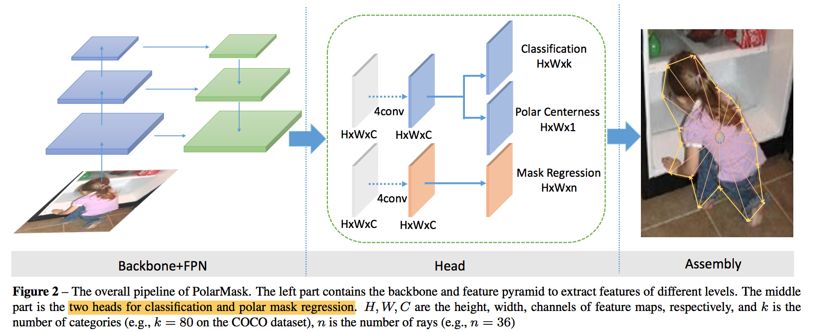
[Pseudo-3D resnet] Learning Spatio-Temporal Representation with Pseudo-3D Residual Networks：伪3d，resblock，S和T花式连接，分类

[2.5d Unet] Automatic Segmentation of Vestibular Schwannoma from T2-Weighted MRI by Deep Spatial Attention with Hardness-Weighted Loss：patch输入，先2d后3d，针对各向异性，分割

[two-pathway U-Net] Combining analysis of multi-parametric MR images into a convolutional neural network: Precise target delineation for vestibular schwannoma treatment planning：patch输入，3d网络，xy和z平面分别conv & concat，分割

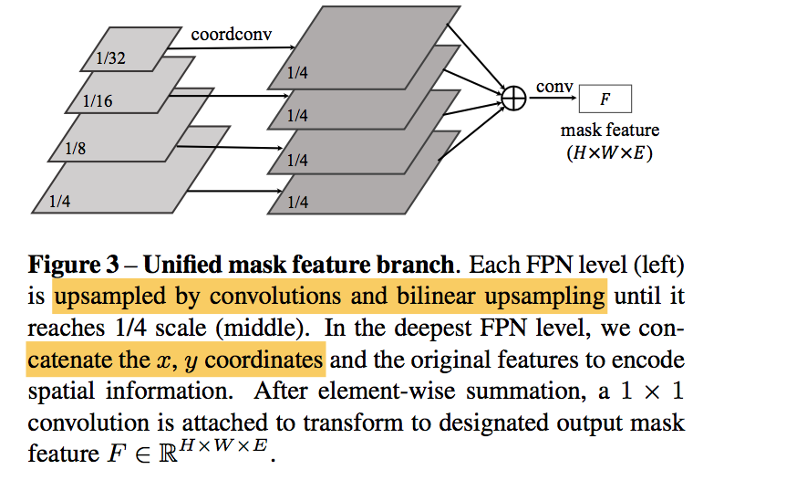
[Projection-Based 2.5D U-net] Projection-Based 2.5D U-net Architecture for Fast Volumetric Segmentation：mip，2d网络，分割，重建

[New 2.5D Representation] A New 2.5D Representation for Lymph Node Detection using Random Sets of Deep Convolutional Neural Network Observations：横冠矢三个平面作为三个channel输入，2d网络，检测

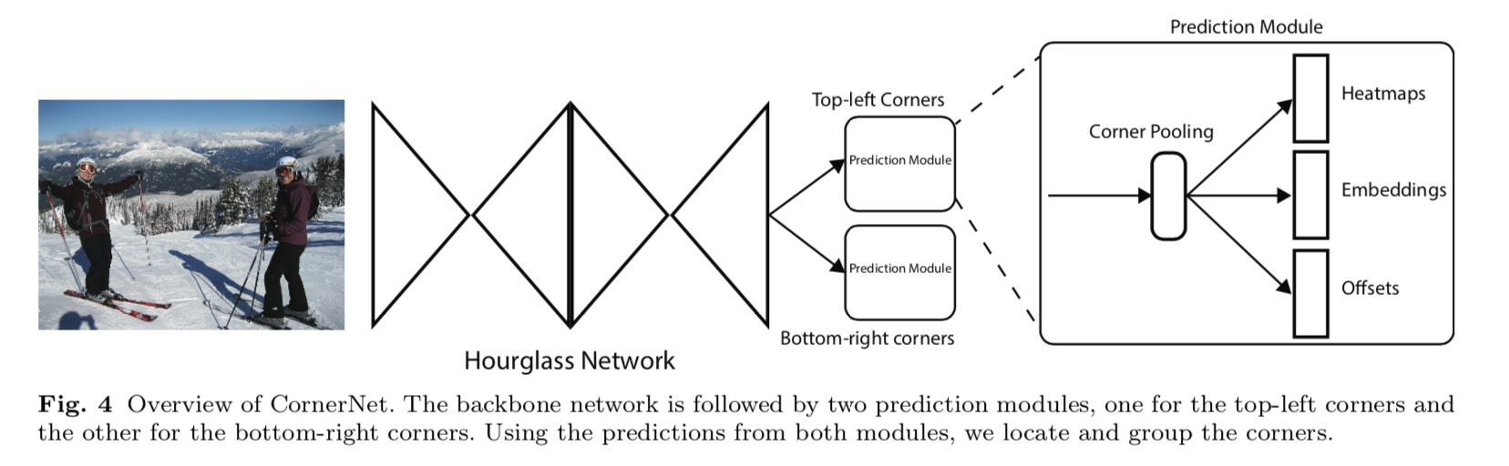
Learning Spatio-Temporal Representation with Pseudo-3D Residual Networks

动机
- spatio-temporal video
- the development of a very deep 3D CNN from scratch results in expensive computational cost and memory demand
- new framework
  - 1x3x3 & 3x1x1
  - Pseudo-3D Residual Net which exploits all the variants of blocks
- outperforms 3D CNN and frame-based 2D CNN
论点
- 3d CNN的model size：making it extremely difficult to train a very deep model
- fine-tuning 2d 好于 train from scrach 3d
- RNN builds only the temporal connections on the high-level features，leaving the correlations in the low-level forms not fully exploited
- we propose
  - 1x3x3 & 3x1x1 in parallel or cascaded
  - 其中的3x3 conv可以用2d conv来初始化
  - a family of bottleneck building blocks：enhance the structural diversity
方法
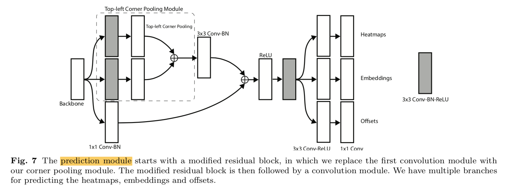
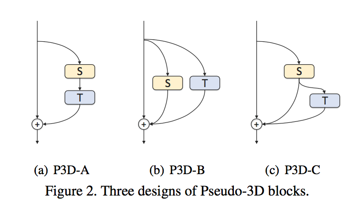
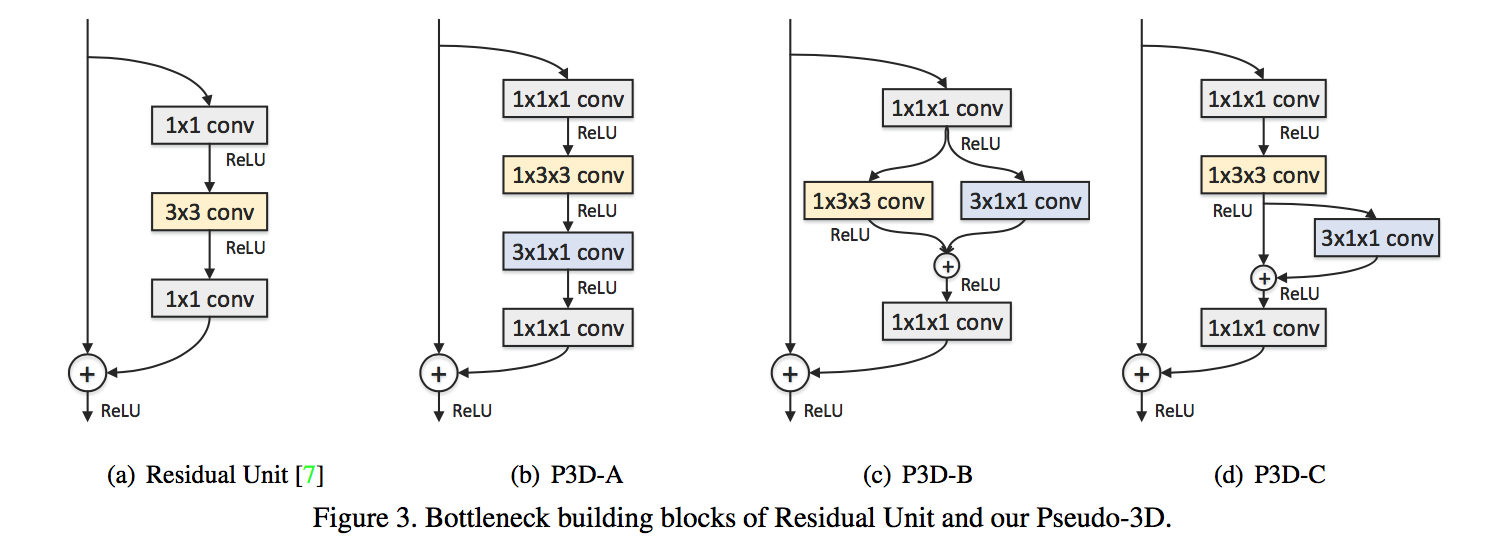
- P3D Blocks
  - direct／indirect influence：S和T之间是串联还是并联
  - direct／indirect connected to the final output：S和T的输出是否直接与identity path相加
  - bottleneck：
    - 头尾各接一个1x1x1的conv
    - 头用来narrow channel，尾用来widen back
    - 头有relu，尾没有relu
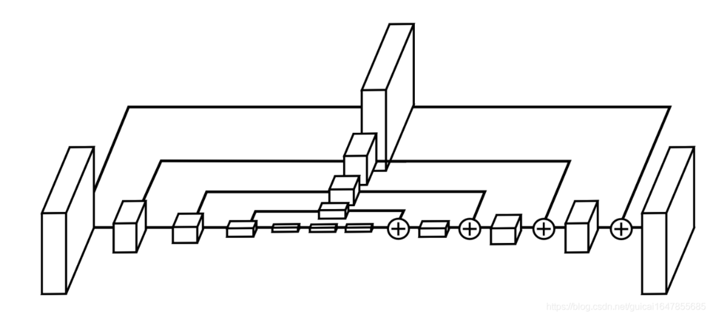
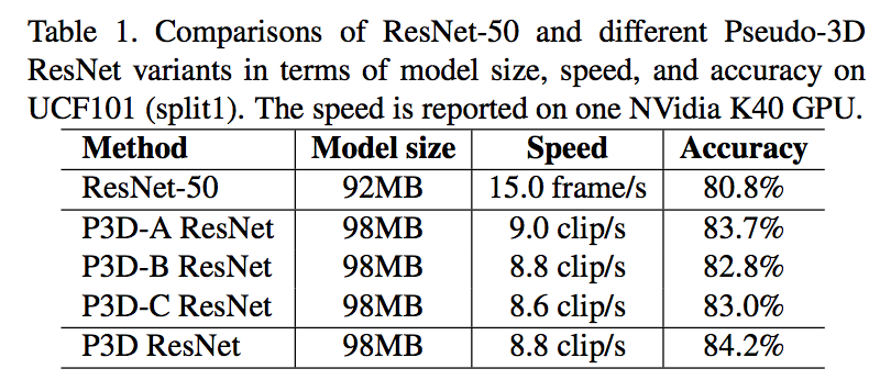
- Pseudo-3D ResNet
  - mixing blocks：循环ABC
  - better performance & small increase in model size
  - fine-tuning resnet50：
    - randomly cropped 224x224
    - freeze all BN except for the first one
    - add an extra dropout layer with 0.9 dropout rate
  - further fine-tuning P3D resnet：
    - initialize with r50 in last step
    - randomly cropped 16x160x160
    - horizontally flipped
    - mini-batch as 128 frames
- future work
  - attention mechanism will be incorporated

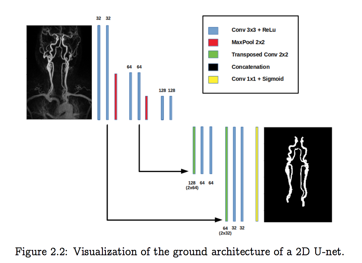
Projection-Based 2.5D U-net Architecture for Fast Volumetric Segmentation

动机
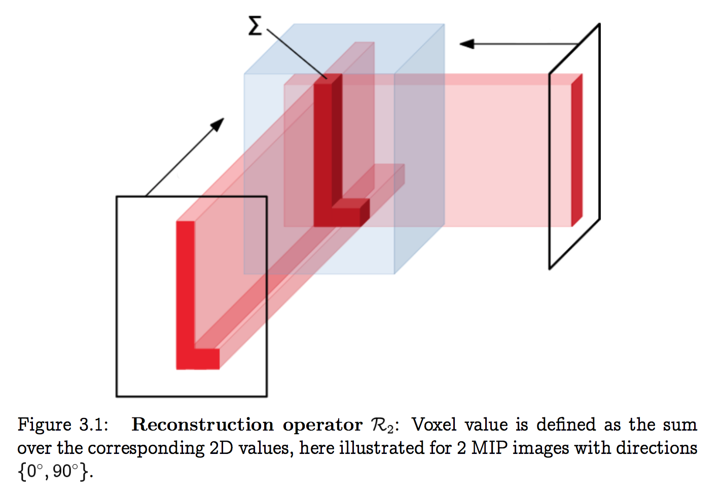
- MIP：2D images containing information of the full 3D image
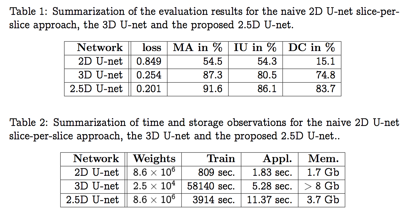
- faster, less memory, accurate
方法
- 2d unet
  - MIP：$\alpha=36$
  - 3x3 conv, s2 pooling, transpose conv, concat, BN, relu,
  - filters：begin with 32, end with 512
  - dropout：0.5 in the deepest convolutional block and 0.2 in the second deepest blocks
- 3d unet
  - overfitting & memory space
  - filters：begin with 4, end with 16
  - dropout：0.5 in the deepest convolutional block and 0.4 in the second deepest blocks
- Projection-Based 2.5D U-net
  - 2d slice：loss of connection
  - 2d mip：disappointing results
  - 2d volume：long training time
  - the proposed 2.5D U-net：
    - $M_{i}$：MIP，p=12
    - $U$：2d-Unet like above
    - $F_p$：learnable filtration，1x3 conv，for each projection，抑制重建伪影
    - $R_p$：reconstruction operator
    - $T$：fine-tuning operator，shift & scale back to 0-1 mask

Learning Spatio-Temporal Features with 3D Residual Networks for Action Recognition

动机
- 3D kernels tend to overfit
- 3D CNNs is relatively shallow
- propose a 3D CNNs based on ResNets
  - better performance
  - not overfit
  - deeper than C3D
论点
- two-stream architecture：consists of RGB and optical flow streams is often used to represent spatio-temporal information
- 3D CNNs：trained on relatively small video datasets performs worse than 2D CNNs pretrained on large datasets
- Very deep 3D CNNs：not explored yet due to training difficulty
方法
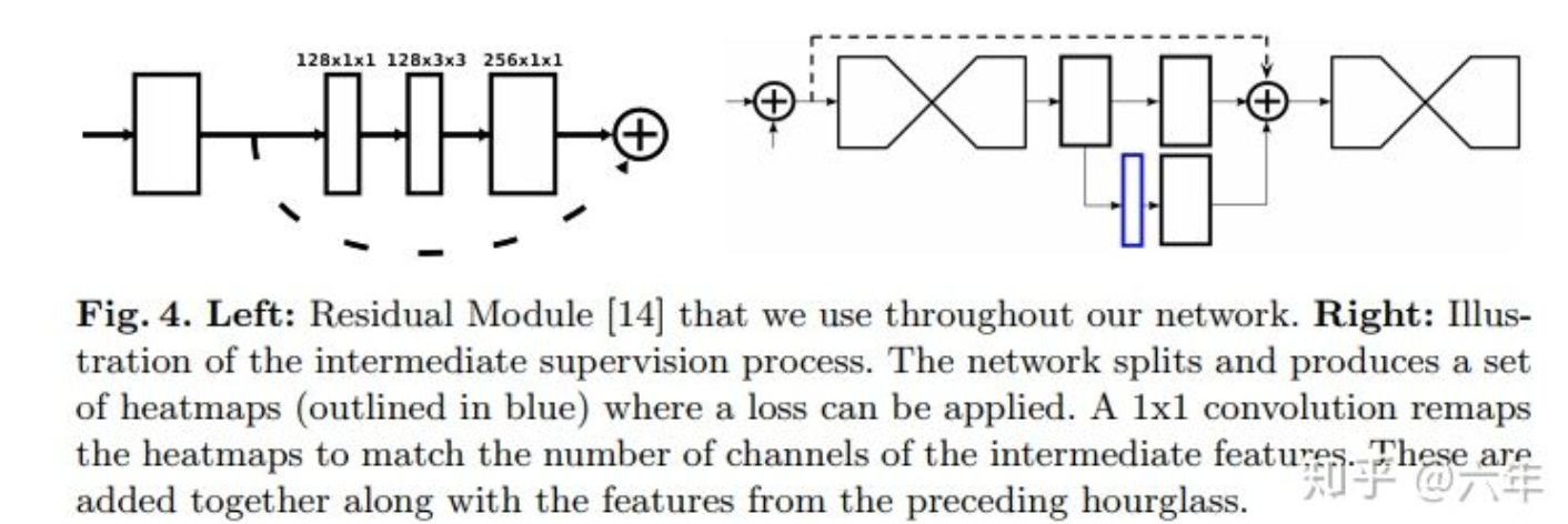
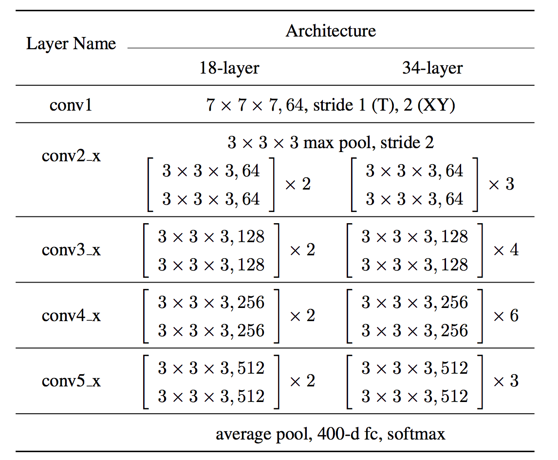
- Network Architecture
  - main difference：kernel dimensions
  - stem：stride2 for S，stride1 for T
  - resblock：conv_bn_relu&conv + id
  - identity shortcuts：use zero-padding for increasing dimensions，to avoid increasing the number of parameters
  - stride2 conv：conv3_1、 conv4_1、 conv5_1
  - input clips：3x16x112x112
  - large learning rate and batch size was important
实验
- 在小数据集上3d-r18不如C3D，overfit了：shallow architecture of the C3D and pretraining on the Sports-1M dataset prevent the C3D from overfitting
- 在大数据集上3d-r34好于C3D，同时C3D的val acc明显高于train acc——太shallow欠拟合了，r34则表现更好，而且不需要预训练
- RGB-I3D achieved the best performance
  - 3d-r34是更deeper的
  - RGB-I3D用了更大的batch size：Large batch size is important to train good models with batch normalization
  - High resolutions：3x64x224x224

Learning Spatiotemporal Features with 3D Convolutional Networks

动机
- generic
- efficient
- simple
- 3d ConvNet with 3x3x3 conv & a simple linear classifier
论点
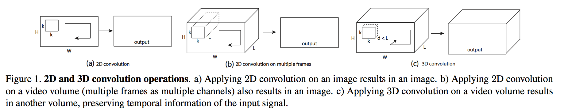
- 3D ConvNets are more suitable for spatiotemporal feature learning compared to 2D ConvNets
- 2D ConvNets lose temporal information of the input signal right after every convolution operation
- 2d conv在channel维度上权重都是一样的，相当于temporal dims上没有重要性特征提取
方法
- basic network settings
  - 5 conv layers + 5 pooling layers + 2 fc layers + softmax
  - filters：[64，128，256，256，256]
  - fc dims：[2048，2048]
  - conv kernel：dx3x3
  - pooling kernel：2x2x2，s2 except for the first layer
    - with the intention of not to merge the temporal signal too early
    - also to satisfy the clip length of 16 frames
- varing settings
  - temporal kernel depth
    - homogeneous：depth-1/3/5/7 throughout
    - varying：increasing-3-3-5-5-7 & decreasing-7- 5-5-3-3
  - depth-3 throughout performs the best
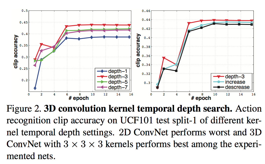
  - depth-1 is significantly worse
  - We also verify that 3D ConvNet consistently performs better than 2D ConvNet on a large-scale internal dataset
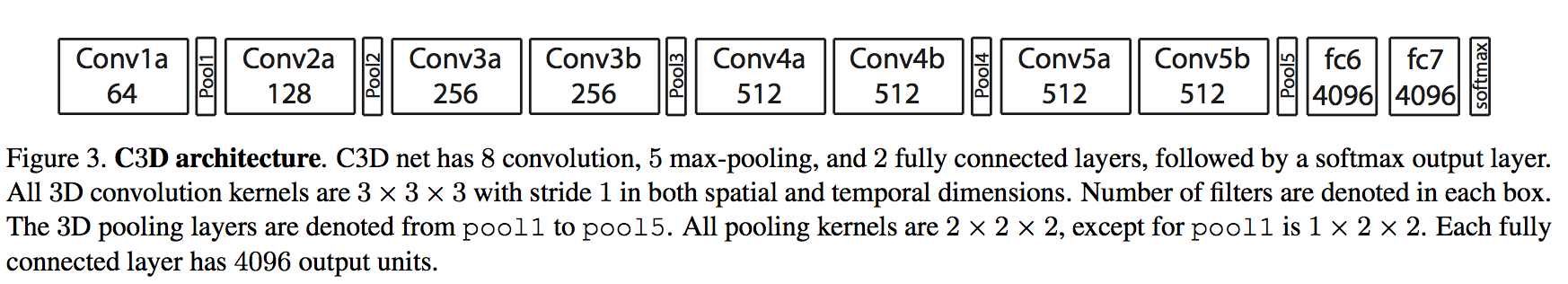
- C3D
  - 8 conv layers + 5 pooling layers + 2 fc layers + softmax
  - homogeneous：3x3x3 s1 conv thtoughout
  - pool1：1x2x2 kernel size & stride，rest 2x2x2
  - fc dims：4096
- C3D video descriptor：fc6 activations + L2-norm
- deconvolution visualizing：
  - conv5b feature maps
  - starts by focusing on appearance in the first few frames
  - tracks the salient motion in the subsequent frames
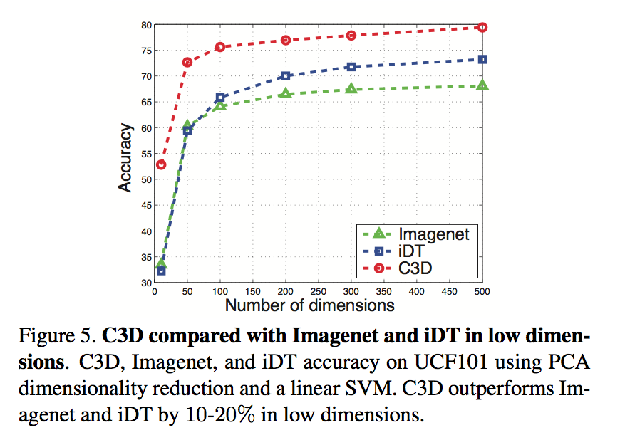
- compactness
  - PCA
  - 压缩到50-100dim不太损失acc
  - 压缩到10dim仍旧是最高acc
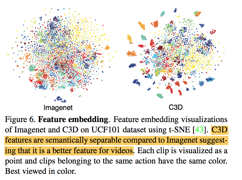
  - projected to 2-dimensional space using t-SNE
    - C3D features are semantically separable compared to Imagenet
    - quantitatively observe that C3D is better than Imagenet
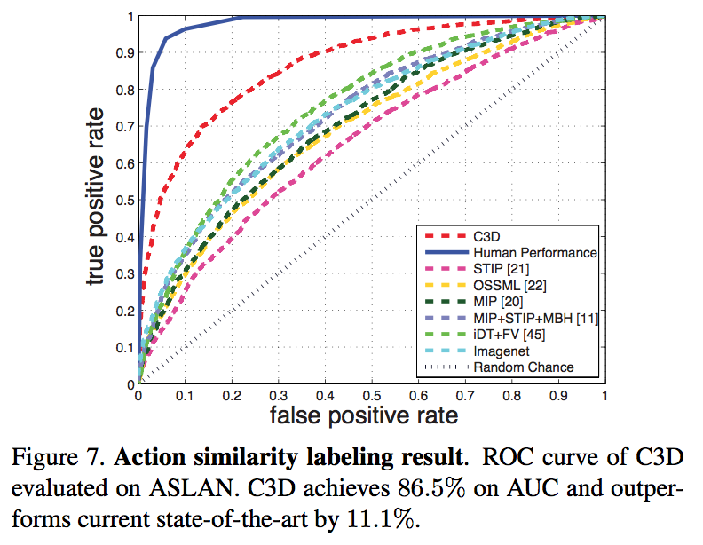
Action Similarity Labeling
- predicting action similarity
- extract C3D features: prob, fc7, fc6, pool5 for each clip
- L2 normalization
- compute the 12 different distances for each feature：48 in total
- linear SVM is trained on these 48-dim feature vectors
- C3D significantly outperforms the others

SSD

发表于 2020-08-13 |

SSD: Single Shot MultiBox Detector

动机
- single network
- speed & accuracy
- 59 FPS / 74.3% mAP
论点
- prev methods
  - two-stage：生成稀疏的候选框，然后对候选框进行分类与回归
  - one-stage：均匀地在图片的不同位置，采用不同尺度和长宽比，进行密集抽样，然后利用CNN提取特征后直接进行分类与回归
- fundamental speed improvement
  - eliminating bounding box proposals
  - eliminating feature resampling
- other improvements
  - small convolutional filter for bbox categories and offsets（针对yolov1的全连接层说）
  - separate predictors by aspect ratio
  - multiple scales
  - 这些操作都不是原创
- The core of SSD is predicting category scores and box offsets for a fixed set of default bounding boxes using small convolutional filters applied to feature maps.
方法
- Model
  - Multi-scale feature maps for detection：采用了多尺度的特征图，逐渐用s2降维，大尺度特征图上有更多的单元，用来回归小物体
  - Convolutional predictors for detection：针对yolov1里面的fc层
  - Default boxes and aspect ratios：一个单元4种size的先验框，对每个先验框都预测一组4+(c+1)，其中的1可以看作背景类，也可以看做是有无目标的置信度，各用一个conv3x3的head
  - backbone
    - 参考：https://www.cnblogs.com/sddai/p/10206929.html
  - VGG16前四个conv block保留
    - 无dropout和fc
    - conv5的池化由2x2-s2变成3x3-s1
    - conv6和conv7是3x3x1024和1x1x1024的空洞卷积，输出19x19x1024
    - conv8是1x1x256和3x3x512 s2的conv，输出10x10x512
    - conv9都是1x1x128和3x3x256 s2的conv，输出5x5x256
    - conv10、conv11都是1x1x128和3x3x256 s1 p0的conv，输出3x3x256、1x1x256
- Training
  - Matching strategy：match default box和gt box
    - 首先为每一个gt box找到一个overlap最大的default box
    - 然后找到所有与gt box的overlap大于0.5的default box
    - 一个gt box可能对应多个default box
    - 一个default box只能对应一个gt box（overlap最大的）
  - Objective loss
    - loc loss：smooth L1，offsets like Faster R-CNN
    - cls loss：softmax loss
    - weighted sum：$L = \frac{1}{N} (L_{cls} + \alpha L_{loc})$，
      - N is the number of matched default boxes
      - loss=0 when N=0
  - Choosing scales and aspect ratios for default boxes
    - 每个level的feature map感受野不同，default box的尺寸也不同
    - 数量也不同，conv4、conv10和conv11是4个，conv7、conv8、conv9是6个
    - ratio：{1,2,3,1/2,1/3}，4个的没有3和1/3
    - L2 normalization for conv4：
      - $y_i = \frac{x_i}{\sqrt{\sum_{k=1}^n x_k^2}}$
      - 作用是将不同尺度的特征都归一化成模为1的向量
      - scale：可以是固定值，也可以是可学习参数
      - 为啥只针对conv4？作者的另一篇paper(ParseNet)中发现conv4和其他层特征的scale是不一样的
  - predictions
    - all default boxes with different scales and aspect ratio from all locations of many feature maps
    - significant imbalance for positive/negative
    - Hard negative mining
      - sort using the highest confidence loss
      - pick the top ones with n/p at most 3:1
      - faster optimization and a more stable training
  - Data augmentation
    - sample a patch with specific IoU
    - resize
性质
- much worse performance on smaller objects, increasing the input size can help improve
- Data augmentation is crucial, resulting in a 8.8% mAP improvement
- Atrous is faster, 保留pool5不变的话，the result is about the same while the speed is about 20% slower

python多线程&多进程

发表于 2020-08-04 |

Reference：

https://www.cnblogs.com/kaituorensheng/p/4465768.html

https://zhuanlan.zhihu.com/p/46368084

https://www.runoob.com/python3/python3-multithreading.html

名词
- 进程(process)和线程(thread)
  - cpu在处理任务时，把时间分成若干个小时间段，这些时间段很小的，系统中有很多进程，每个进程中又包含很多线程，在同一时间段内，电脑CPU只能处理一个线程，下一个时间段，可能又去执行别的线程了（时间片轮转，从而实现伪多任务），具体顺序取决于其调度逻辑
  - 多核cpu可以实现真正的并行，同一个时刻每个cpu上都可以跑一个任务
  - 多进程：每个进程分别执行指定任务，进程间互相独立，每个时刻并行的实际进程数取决于cpu数量
  - 多线程：单个cpu同一时刻只能处理一个线程，一个任务可能由多个工人来完成，工人们相互协同，这则是多线程
- python的多进程：multiprocess模块
- python的多线程：threading模块
- 每个进程在执行过程中拥有独立的内存单元，而一个进程的多个线程在执行过程中共享内存。
多进程multiprocess
- 母进程：当我们执行一个python脚本，if main下面实际运行的主体就是母进程
- 子进程：我们使用multiprocess显式创建的进程，都是子进程
- join()方法：用来让母进程阻塞，等待所有子进程执行完成再结束

使用multiprocess的多进程，可以通过process方法和pool方法
- process方法：适用进程较少时候，无法批量开启/关闭
- pool方法：批量管理
- 参数：输入参数都差不多，第一个是要执行的函数方法target/func，第二个是输入参数args

🌰Process方法：

from multiprocessing import Process
import os
import time


def long_time_task(i):
    print('子进程: {} - 任务{}'.format(os.getpid(), i))
    time.sleep(2)
    print("结果: {}".format(8 ** 20))


if __name__=='__main__':
    print('当前母进程: {}'.format(os.getpid()))
    start = time.time()
    p1 = Process(target=long_time_task, args=(1,))
    p2 = Process(target=long_time_task, args=(2,))
    print('等待所有子进程完成。')
    p1.start()
    p2.start()
    p1.join()
    p2.join()
    end = time.time()
    print("总共用时{}秒".format((end - start)))

process方法使用Process实例化一个进程对象，然后调用它的start方法开启进程

🌰Pool方法：

from multiprocessing import Pool, cpu_count
import os
import time


def long_time_task(i):
    print('子进程: {} - 任务{}'.format(os.getpid(), i))
    time.sleep(2)
    print("结果: {}".format(8 ** 20))
    return True     # 用于演示pool适用于有返回值


if __name__=='__main__':
    print("CPU内核数:{}".format(cpu_count()))        # 4
    print('当前母进程: {}'.format(os.getpid()))
    start = time.time()
    p = Pool(4)
    results = []
    for i in range(5):
        # p.apply_async(long_time_task, args=(i,))
        results.append(p.apply_async(long_time_task, args=(i,)))
    print('等待所有子进程完成。')
    p.close()
    p.join()
    end = time.time()
    print("总共用时{}秒".format((send - start)))
    
    # 查看返回值
    for res in results:
      print(res.get())

apply_async(func, args=(), kwds={}, callback=None)：向进程池提交需要执行的函数及参数，各个进程采用非阻塞（异步）的调用方式，即每个子进程只管运行自己的，不管其它进程是否已经完成。
close()：关闭进程池（pool），不再接受新的任务。
join()：主进程阻塞等待子进程的退出，调用join()之前必须先调用close()或terminate()方法，使其不再接受新的Process。

多线程threading

python的多线程是伪多线程，因为主进程只有一个，所以只用了单核，只是通过碎片化进程、调度、全局锁等操作，cpu利用率提升了
所以我想并行处理百万量级的数据入库操作时，多进程的效率明显高于多线程

【问题】从我观察上看多线程基本就是串行？？

🌰threading

import threading
import time


def long_time_task():
    print('当子线程: {}'.format(threading.current_thread().name))
    time.sleep(2)
    print("结果: {}".format(8 ** 20))


if __name__=='__main__':
    start = time.time()
    print('这是主线程：{}'.format(threading.current_thread().name))
    for i in range(5):
        t = threading.Thread(target=long_time_task, args=())
        t.setDaemon(True)
        t.start()
        t.join()

    end = time.time()
    print("总共用时{}秒".format((end - start)))
    
    
# 继承&有返回值的写法
def long_time_task(i):
    time.sleep(2)
    return 8**20


class MyThread(threading.Thread):
    def __init__(self, func, args , name='', ):
        threading.Thread.__init__(self)
        self.func = func
        self.args = args
        self.name = name
        self.result = None

    def run(self):
        print('开始子进程{}'.format(self.name))
        self.result = self.func(self.args[0],)
        print("结果: {}".format(self.result))
        print('结束子进程{}'.format(self.name))
    def get_result(self):
        threading.Thread.join(self)  # 等待线程执行完毕
        return self.result

if __name__=='__main__':
    start = time.time()
    threads = []
    for i in range(1, 3):
        t = MyThread(long_time_task, (i,), str(i))
        threads.append(t)

    for t in threads:
        t.start()
    for t in threads:
        t.join()

    end = time.time()
    print("总共用时{}秒".format((end - start)))

join方法：等待所有进程执行完，主进程再执行完
setDaemon(True)：主线程执行完就退出

IoU

发表于 2020-08-03 |

reference: https://bbs.cvmart.net/articles/1396

IoU

IoU = Intersection / Union

$Loss_{IoU} = 1 - IoU$
- [0,1]
- 无法直接优化没有重叠的部分：如果两个框没有交集，IoU=0，没有梯度回传，无法进行学习训练
- 尺度不敏感
- 无法精确的反映两者的重合质量
GIoU(Generalized Intersection over Union)

$GIoU = IoU - \frac{|A_c - U|}{|A_c|}$，$A_c$是包含两个框的最小外接框

$Loss_{GIoU} = 1 - GIoU$
- GIoU倾向于先增大bbox的大小来增大与GT的交集，然后通过IoU项引导最大化bbox的重叠区域
- [-1,1]：对称区间
- 能够关注到非重合区域：引入了外接框C
- 尺度不敏感
- 两个框为包含关系时，退化为IoU
- 如果之间用来替换mse，前期收敛会比较慢
- 一般地，GIoU loss不能很好地收敛SOTA算法，反而造成不好的结果
DIoU (Distance-IoU)

$DIoU = IoU - \frac{d^2}{c^2}$，d是两个中心点间的欧式距离，c是两个框的最小外接框的对角线距离

$Loss_{DIoU} = 1 - DIoU$

* 直接最小化两个目标框的距离，收敛快得多，而且稳定

* 也能够关注到非重合区域：引入外接对角线

* 对于包含关系的两个框，仍旧有距离损失，不会退化为IoU：因为中心点距离

* 可以替换NMS中的IoU：原始的IoU仅考虑了重叠区域，对包含的情况没有很好的处理
    $$
    score = score\text{ if }IoU - dis(box_{max}, box)>\epsilon \text{, else } 0
    $$

* 没有考虑形状（长宽比）

CIoU (Complete-IoU)

$CIoU = IoU - \frac{d^2}{c^2}-av$，在DIoU的基础上新增了惩罚项av，a是权重系数，v用来评价长宽比：

$Loss_{CIoU} = 1 - CIoU$
- v的梯度中有$\frac{1}{w^2+h^2}$，长宽在[0,1]之间，可能很小，会导致梯度爆炸，用的时候
  - clamp一下上下限
  - 分母中的$w^2+h^2$替换成1
    $\frac{\partial v }{\partial w} = \frac{8}{\pi ^ 2}(arctan\frac{w^{gt}}{h^{gt}}-arctan\frac{w}{h})\frac{h}{w^2+h^2}\\ \frac{\partial v }{\partial w} = \frac{8}{\pi ^ 2}(arctan\frac{w^{gt}}{h^{gt}}-arctan\frac{w}{h})\frac{w}{w^2+h^2}$

YOLOACT

发表于 2020-07-17 |

[YOLACT] Real-time Instance Segmentation：33 FPS/30 mAP
[YOLACT++] Better Real-time Instance Segmentation：33.5 FPS/34.1 mAP

YOLACT: Real-time Instance Segmentation

动机
- create a real-time instance segmentation base on fast, one-stage detection model
- forgoes an explicit localization step (e.g., feature repooling)
  - doesn’t depend on repooling (RoI Pooling)
  - produces very high-quality masks
- set two parallel subtasks
  - prototypes——conv
  - mask coefficients——fc
  - 之后将模板mask和实例mask系数进行线性组合来获得实例的mask

‘prototypes’: vocabulary
fully-convolutional
- localization is still translation variant
Fast NMS

论点
- State-of-the-art approaches to instance segmentation like Mask R- CNN and FCIS directly build off of advances in object detection like Faster R-CNNand R-FCN
  - focus primarily on performance over speed
  - these methods “re-pool” features in some bounding box region
  - inherently sequential therefore difficult to accelerate
- One-stage instance segmentation methods generate position sensitive maps
  - still require repooling or other non-trivial computations
- prototypes
  - related works use prototypes to represent features (Bag of Feature)
  - we use them to assemble masks for instance segmentation
  - we learn prototypes that are specific to each image, rather than global prototypes shared across the entire dataset
- Bag of Feature
  - BOF假设图像相当于一个文本，图像中的不同局部区域或特征可以看作是构成图像的词汇(codebook)
  - 所有的样本共享一份词汇本，针对每个图像，统计每个单词的频次，即可得到图片的特征向量
方法
- parallel tasks
  - The first branch uses an FCN to produce a set of image-sized “prototype masks” that do not depend on any one instance.
  - The second adds an extra head to the object detection branch to predict a vector of “mask coefficients” for each anchor that encode an instance’s rep- resentation in the prototype space.
  - linearly combining
- Rationale
  - masks are spatially coherent：mash是空间相关的，相邻像素很可能是一类
  - 卷积层能够利用到这种空间相关性，但是fc层不能
  - 而one-stage检测器的检测头通常是fc层？？
  - making use of fc layers, which are good at producing semantic vectors
  - and conv layers, which are good at producing spatially coherent masks
- Prototype
  - 在backbone feature layer P3上接一个FCN
    - taking protonet from deeper backbone features produces more robust masks
    - higher resolution prototypes result in both higher quality masks and better performance on smaller objects
    - upsample到x4的尺度to increase performance on small objects
  - head包含k个channels
    - 梯度回传来源于最终的final assembled mask，不是当前这个头
    - unbounded：ReLU or no nonlinearity
    - We choose ReLU for more interpretable prototypes
- Mask Coefficients
  - a third branch in parallel with detection heads
  - nonlinearity：要有正负，所以tanh
- Mask Assembly
  - linear combination + sigmoid: $M=\sigma(PC^T)$
  - loss
    - cls loss：w=1, 和ssd一样，c+1 softmax
    - box reg loss：w=1.5, 和ssd一样，smooth-L1
    - mask loss：w=6.125， BCE
  - crop mask
    - eval：用predict box去crop
    - train：用gt box去crop，同时还要给mask loss除以gt box的面积，to preserve small objects
- Emergent Behavior
  - 不crop也能分割中大目标：
    - YOLACT learns how to localize instances on its own via different activations in its prototypes
    - 而不是靠定位结果
  - translation variant
    - the consistent rim of padding in modern FCNs like ResNet gives the network the ability to tell how far away from the image’s edge a pixel is，所以用一张纯色的图能够看出kernel实际highlight的是哪部分特征
    - 同一种kernel，同一种五角星，在画面不同位置，对应的响应值是不同的，说明fcn是能够提取物体位置这样的语义信息的
    - prototypes are compressible：
      - 增加模版数目反而不太有效，because predicting coefficients is difficult，
      - the network has to play a balancing act to produce the right coef- ficients, and adding more prototypes makes this harder,
      - We choose 32 for its mix of performance and speed
- Network
  - speed as well as feature richness
  - backbone参考RetinaNet，ResNet-101 + FPN
    - 550x550 input，resize
    - 去掉P2，add P6&P7
    - 3 anchors per level，[1, 1/2, 2]
    - P3的anchor尺寸是24x24，接下来每层double the scale
    - 检测头：shared conv+parallel conv
    - OHEM
  - single GPU：batch size 8 using ImageNet weights，no extra bn layers
- Fast NMS
  - 构造cxnxn的矩阵，c代表每个class
  - 然后搞成上三角，求column-wise max
  - 再IoU threshold
  - 15.0 ms faster with a performance loss of 0.3 mAP
- Semantic Segmentation Loss
  - using modules not executed at test time
  - P3上1x1 conv，sigmoid and c channels
  - w=1
  - +0.4 mAP boost

YOLACT++: Better Real-time Instance Segmentation

cornerNet

发表于 2020-07-17 |

CornerNet: Detecting Objects as Paired Keypoints

动机
- corner formulation
  - top-left corner
  - bottom-right corner
- anchor-free
- corner pooling
- no multi-scale
论点
- anchor box drawbacks
  - huge set of anchors boxes to ensure sufficient overlap，cause huge imbalance
  - hyperparameters and design choices
- cornerNet
  - detect and group
    - heatmap to predict corners
      - 从数学表达上看，全图wh个tl corner，wh个bt corner，可以表达wwhh个框
    - anchor-based，全图wh个中心点，9个anchor size，只能表达有限的框，且可能match不上
    - embeddings to group pairs of corners
  - corner pooling
    - better localize corners which are usually out of the foreground
  - modifid hourglass architecture
  - add our novel variant of focal loss
方法
- two prediction modules
  - heatmaps
    - C channels, C for number of categories
    - binary mask
    - each corner has only one ground-truth positive
    - penalty the neighbored negatives within a radius that still hold high iou (0.3 iou)
      - determine the radius
      - penalty reduction $=e^{-\frac{x^2+y^2}{2\sigma^2}}$
    - variant focal loss
      - $L_{det} = \frac{-1}{N} \sum^C \sum^H \sum^W \begin{cases} (1-p_{i,j})^\alpha log(p_{i,j}), \ \ if y_{ij}=1\\ (1-y_{ij})^\beta (p_{i,j})^\alpha log(1-p_{i,j}), \ \ otherwise \end{cases}$
      - $\alpha=2, \beta=4$
      - N is the number of gts
  - embeddings
    - associative embedding
    - use 1-dimension embedding
    - pull and push loss on gt positives
      - $L_{pull} = \frac{1}{N} \sum^N [(e_{tk}-e_k)^2 + (e_{bk}-e_k)^2]$
      - $L_{push} = \frac{1}{N(N-1)} \sum_j^N\sum_{k\neq j}^N max(0, \Delta -|e_k-e_j|)$
      - $e_k$ is the average of $e_{tk}$ and $e{bk}$
      - $\Delta$ = 1
  - offsets
    - 从heatmap resolution remapping到origin resolution存在精度损失 $o_k = （\frac{x_k}{n} - \lfloor \frac{x_k}{n} \rfloor， \frac{y_k}{n} - \lfloor \frac{y_k}{n} \rfloor）$
- greatly affect the IoU of small bounding boxes
- shared among all categories
- smooth L1 loss on gt positives
```
      $$
      L_{off} = \frac{1}{N} \sum^N SmoothL1(o_k, \hat o_k)
```
  $$
- corner pooling
  - top-left pooling layer：
```
  * 从当前点(i,j)开始，
  * 向下elementwise max所有feature vecor，得到$t_{i,j}$
  * 向右elementwise max所有feature vecor，得到$l_{i,j}$
  * 最后两个vector相加
```
    - bottom-right corner：向左向上
- Hourglass Network
  - hourglass modules
    - series of convolution and max pooling layers
    - series of upsampling and convolution layers
    - skip layers
  - multiple hourglass modules stacked：reprocess the features to capture higher-level information
  - intermediate supervision
    - 常规的中继监督：
      
      下一级hourglass module的输入包括三个部分
      - 前一级输入
      - 前一级输出
      - 中继监督的输出
    - 本文使用了中继监督，但是没把这个结果加回去
      - hourglass2 input：1x1 conv-BN to both input and output of hourglass1 + add + relu
- Our backbone
  - 2 hourglasses
  - 5 times downsamp with channels [256,384,384,384,512]
  - use stride2 conv instead of max-pooling
  - upsamp：2 residual modules + nearest neighbor upsampling
  - skip connection: 2 residual modules，add
  - mid connection: 4 residual modules
  - stem: 7x7 stride2, ch128 + residual stride2, ch256
  - hourglass2 input：1x1 conv-BN to both input and output of hourglass1 + add + relu
实验
- training details
  - randomly initialized, no pretrained
  - bias：set the biases in the convolution layers that predict the corner heatmaps
  - input：511x511
  - output：128x128
  - apply PCA to the input image
  - full loss：$L = L_{det} + \alpha L_{pull} + \beta L_{push} + \gamma L_{off}$
    - 配对loss：$\alpha=\beta=0.1$
    - offset loss：$\gamma=1$
  - batch size = 49 = 4+5x9
- test details
  - NMS：3x3 max pooling on heatmaps
  - pick：top100 top-left corners & top100 bottom-right corners
  - filter pairs：
    - L1 distance greater than 0.5
    - from different categories
  - fusion：combine the detections from the original and flipped images + soft nms
- Ablation Study
  - corner pooling is especially helpful for medium and large objects
  - penalty reduction especially benefits medium and large objects
  - CornerNet achieves a much higher AP at 0.9 IoU than other detectors：更有能力生成高质量框
  - error analysis：the main bottleneck is detecting corners

CornerNet-Lite: Efficient Keypoint-Based Object Detection

动机
- keypoint-based methods
  - detecting and grouping
  - accuary but with processing cost
- propose CornerNet-Lite
  - CornerNet-Saccade：attention mechanism
  - CornerNet-Squeeze：a new compact backbone
- performance
论点
- main drawback of cornerNet
  - inference speed
  - reducing the number of scales or the image resolution cause a large accuracy drop
- two orthogonal directions
  - reduce the number of pixels to process：CornerNet-Saccade
  - reduce the amount of processing per pixel：
- CornerNet-Saccade
  - downsized attention map
  - select a subset of crops to examine in high resolution
  - for off-line：AP of 43.2% at 190ms per image
- CornerNet-Squeeze
  - inspired by squeezeNet and mobileNet
  - 1x1 convs
  - bottleneck layers
  - depth-wise separable convolution
  - for real-time：AP of 34.4% at 30ms
- combined??
  - CornerNet-Squeeze-Saccade turns out slower and less accurate than CornerNet- Squeeze
- Saccades：扫视
  - to generate interesting crops
  - RCNN系列：single-type & single object
  - AutoFocus：add a branch调用faster-RCNN，thus multi-type & mixed-objects，有single branch有multi branch
  - CornerNet-Saccade：
    - single-type & multi object
    - crops can be much smaller than number of objects
方法
- CornerNet-Saccade
  - step1：obtain possible locations
    - downsize：two scales，255 & 192，zero-padding
    - predicts 3 attention maps
      - small object：longer side<32 pixels
      - medium object：32-96
      - large object：>96
      - so that we can control the zoom-in factor：zoom-in more for smaller objects
      - feature map：different scales from the upsampling layers
      - attention map：3x3 conv-relu + 1x1 conv-sigmoid
      - process locations where scores > 0.3
  - step2：finer detection
    - zoom-in scales：4，2，1 for small、medium、large objects
    - apply CornerNet-Saccade on the ROI
      - 255x255 window
      - centered at the location
  - step3：NMS
    - soft-nms
    - remove the bounding boxes which touch the crop boundary
  - CornerNet-Saccade uses the same network for attention maps and bounding boxes
    - 在第一步的时候，对一些大目标已经有了检测框
    - 也要zoom-in，矫正一下
  - efficiency
    - regions/croped images都是processed in batch/parallel
    - resize/crop操作在GPU中实现
    - suppress redundant regions using a NMS-similar policy before prediction
- new hourglass backbone
  - 3 hourglass module，depth 54
  - downsize twice before hourglass modules
  - downsize 3 times in each module，with channels [384,384,512]
  - one residual in both encoding path & skip connection
  - mid connection：one residual，with channels 512
- CornerNet-Squeeze
  - to replace the heavy hourglass104
  - use fire module to replace residuals
  - downsizes 3 times before hourglass modules
  - downsize 4 times in each module
  - replace the 3x3 conv in prediction head with 1x1 conv
  - replace the nearest neighboor upsampling with 4x4 transpose conv

SOLO

发表于 2020-07-17 |

[SOLO] SOLO: Segmenting Objects by Locations：字节，目前绝大多数方法实例分割的结构都是间接得到——检测框内语义分割／全图语义分割聚类，主要原因是formulation issue，很难把实例分割定义成一个结构化的问题

[SOLOv2] SOLOv2: Dynamic, Faster and Stronger：best 41.7% AP

SOLO: Segmenting Objects by Locations

动机
- challenging：arbitrary number of instances
- form the task into a classification-solvable problem
- direct & end-to-end & one-stage & using mask annotations solely
- on par accuracy with Mask R-CNN
- outperforming recent single-shot instance segmenters
论点
- formulating
  - Objects in an image belong to a fixed set of semantic categories——semantic segmentation can be easily formulated as a dense per-pixel classification problem
  - the number of instances varies
- existing methods
  - 检测／聚类：step-wise and indirect
  - 累积误差
- core idea
  - in most cases two instances in an image either have different center locations or have different object sizes
  - location：
    - think image as a divided grid of cells
    - an object instance is assigned to one of the grid cells as its center location category
    - encode center location categories as the channel axis
  - size
    - FPN
    - assign objects of different sizes to different levels of feature maps
  - SOLO converts coordinate regression into classification by discrete quantization
  - One feat of doing so is the avoidance of heuristic coordination normalization and log-transformation typically used in detectors【？？？不懂这句话想表达啥】
方法
- problem formulation
  - divided grids
  - simultaneous task
    - category-aware prediction
    - instance-aware mask generation
  - category prediction
    - predict instance for each grid：$SSC$
    - grid size：$S*S$
    - number of classes：$C$
    - based on the assumption that each cell must belong to one individual instance
    - C-dim vec indicates the class probability for each object instance in each grid
  - mask prediction
    - predict instance mask for each positive cell：$HWS^2$
    - the channel corresponding to the location
    - position sensitive：因为每个grid中分割的mask是要映射到对应的channel的，因此我们希望特征图是spatially variant
      - 让特征图spatially variant的最直接办法就是加一维spatially variant的信息
      - inspired by CoordConv：添加两个通道，normed_x和normed_y，[-1,1]
      - original feature tensor $HWD$ becomes $HW(D+2)$
  - final results
    - gather category prediction & mask prediction
    - NMS
- network
  - backbone：resnet
  - FCN：256-d
  - heads：weights are shared across different levels except for the last 1x1 conv
- learning
  - positive grid：falls into a center region
    - mask：mask center $(c_x, c_y)$，mask size $(h,w)$
    - center region：$(c_x,c_y,\epsilon w, \epsilon h)$，set $\epsilon = 0.2$
  - loss：$L = L_{cate} + \lambda L_{seg}$
    - cate loss：focal loss
    - seg loss：dice，$L_{mask} = \frac{1}{N_{pos}}\sum_k 1_{p^_{i,j}>0} dice(m_k, m^_k) $，带星号的是groud truth
- inference
  - use a confidence threshold of 0.1 to filter out low spacial predictions
  - use a threshold of 0.5 to binary the soft masks
  - select the top 500 scoring masks
  - NMS
    - Only one instance will be activated at each grid
    - and one in- stance may be predicted by multiple adjacent mask channels
  - keep top 100
实验
- grid number
  - 适当增加有提升，主要提升还是在FPN
- fpn
  - 五个FPN pyramids
  - 大特征图，小感受野，用来分配小目标，grid数量要增大
- feature alignment
  - 在分类branch，$HW$特征图要转换成$SS$的特征图
    - interpolation：bilinear interpolating
    - adaptive-pool：apply a 2D adaptive max-pool
    - region-grid- interpolation：对每个cell，采样多个点做双线性插值，然后取平均
  - is no noticeable performance gap between these variants
  - （可能因为最终是分类任务
- head depth
  - 4-7有涨点
  - 所以本文选了7
decoupled SOLO
- mask branch预测的channel数是$S^2$，其中大部分channel其实是没有贡献的，空占内存
- prediction is somewhat redundant as in most cases the objects are located sparsely in the image
- element-wise multiplication
- 实验下来
  - achieves the same performance
  - efficient and equivalent variant

SOLOv2: Dynamic, Faster and Stronger

动机
- take one step further on the mask head
  - dynamically learning the mask head
  - decoupled into mask kernel branch and mask feature branch
- propose Matrix NMS
  - faster & better results
- try object detection and panoptic segmentation
论点
- SOLO develop pure instance segmentation
- instance segmentation
  - requires instance-level and pixel-level predictions simultaneously
  - most existing instance segmentation methods build on the top of bounding boxes
  - SOLO develop pure instance segmentation
- SOLOv2 improve SOLO
  - mask learning：dynamic scheme
  - mask NMS：parallel matrix operations，outperforms Fast NMS
- Dynamic Convolutions
  - STN：adaptively transform feature maps conditioned on the input
  - Deformable Convolutional Networks：learn location
方法
- revisit SOLOv1
  - redundant mask prediction
  - decouple
  - dynamic：dynamically pick the valid ones from predicted $s^2$ classifiers and perform the convolution
- SOLOv2
  - dynamic mask segmentation head
    - mask kernel branch
    - mask feature branch
  - mask kernel branch
    - prediction heads：4 convs + 1 final conv，shared across scale
    - no activation on the output
    - concat normalized coordinates in two additional input channels at start
    - ouputs D-dims kernel weights for each grid：e.g. for 3x3 conv with E input channels, outputs $SS9E$
  - mask feature branch
    - predict instance-aware feature：$F \in R^{HWE}$
    - unified and high-resolution mask feature：只输出一个尺度的特征图，encoded x32 feature with coordinates info
      - we feed normalized pixel coordinates to the deepest FPN level (at 1/32 scale)
      - repeated 【3x3 conv, group norm, ReLU, 2x bilinear upsampling】
      - element-wise sum
      - last layer：1x1 conv, group norm, ReLU
  - instance mask
    - mask feature branch conved by the mask kernel branch：final conv $HWS^2$
    - mask NMS
  - train
    - loss：$L = L_{cate} + \lambda L_{seg}$
      - cate loss：focal loss
      - seg loss：dice，$L_{mask} = \frac{1}{N_{pos}}\sum_k 1_{p^_{i,j}>0} dice(m_k, m^_k) $，带星号的是groud truth
  - inference
    - category score：first use a confidence threshold of 0.1 to filter out predictions with low confidence
    - mask branch：run convolution based on the filtered category map
    - sigmoid
    - use a threshold of 0.5 to convert predicted soft masks to binary masks
    - Matrix NMS
  - Matrix NMS
    - decremented functions
      - linear：$f(iou_{i,j}=1-iou_{i,j})$
      - gaussian：$f(iou_{i,j}=exp(-\frac{iou_{i,j}^2}{\sigma})$
    - the most overlapped prediction for $m_i$：max iou
      - $f(iou_{*,i}) = min_{s_k}f(iou_{k,i})$
    - decay factor
      - $decay_i = min \frac{f(iou_{i,j})}{f(iou_{*,i})}$

polarMask

发表于 2020-06-29 |

PolarMask: Single Shot Instance Segmentation with Polar Representation

动机
- instance segmentation
- anchor-free
- single-shot
- modified on FCOS
论点
- two-stage methods
  - FCIS, Mask R-CNN
  - bounding box detection then semantic segmentation within each box
- single-shot method
  - formulate the task as instance center classification and dense distance regression in a polar coordinate
  - FCOS can be regarded as a special case that the contours has only 4 directions
- this paper
  - two parallel task：
    - instance center classification
    - dense distance regression
  - Polar IoU Loss can largely ease the optimization and considerably improve the accuary
  - Polar Centerness improves the original idea of “Centreness” in FCOS, leading to further performance boost
方法
- architecture
  - back & fpn are the same as FCOS
  - model the instance mask as one center and n rays
    - conclude that mass-center is more advantageous than box center
    - the angle interval is pre-fixed, thus only the length of the rays is to be regressed
    - positive samples：falls into 1.5xstrides of the area around the gt mass-center，that is 9-16 pixels around gt grid
    - distance regression
      - 如果一条射线上存在多个交点，取最长的
      - 如果一条射线上没有交点，取最小值$\epsilon=10^{-6}$
- potential issuse of the mask regression branch
  - dense regression task with such as 36 rays, may cause imbalance between regression loss and classification loss
  - n rays are relevant and should be trained as a whole rather than a set of independent values—->iou loss
- inference
  - multiply center-ness with classification to obtain final confidence scores, conf thresh=0.05
  - take top-1k predictions per fpn level
  - use the smallest bounding boxes to run NMS, nms thresh=0.5
- polar centerness
  - to suppress low quality detected centers
  - $polar\ centerness=\sqrt{\frac{min(\{d_1,d_2, …, d_n\})}{max(\{d_1,d_2, …, d_n\})}}$
  - $d_{min}$和$d_{max}$越接近，说明中心点质量越好
  - Experiments show that Polar Centerness improves accuracy especially under stricter localization metrics, such as $AP_{75}$
- polar IoU loss
  - polar IoU：$IoU=lim_{N\to\inf}\frac{\sum_{i=1}^N\frac{1}{2} d_{min}^2 \Delta \theta}{\sum_{i=1}^N\frac{1}{2} d_{max}^2 \Delta \theta}$
  - empirically observe that 去掉平方项效果更好：$polar\ IoU=\frac{\sum_{i=1}^n d_{min}}{\sum_{i=1}^n d_{max}}$
  - polar iou loss：bce of polar IoU，$-log(\frac{\sum_{i=1}^n d_{min}}{\sum_{i=1}^n d_{max}})$
  - advantage
    - differentiable, enable bp
    - regards the regression targets as a whole
    - keep balance with classification loss

FCOS

发表于 2020-06-23 |

FCOS: Fully Convolutional One-Stage Object Detection

动机
- anchor free
- proposal free
- avoids the complicated computation related to anchor boxes
  - calculating overlapping during training
- avoid all hyper-parameters related to anchor boxes
  - size & shape
  - positive／ignored／negative
- leverage as many foreground samples as possible
论点
- anchor-based detectors
  - detection performance is sensitive to anchor settings
  - encounter difficulties in cases with large shape variations
  - hamper the generalization ability of detectors
  - dense propose：the excessive number of negative samples aggravates the imbalance
  - involve complicated computation：such as calculating the IoU with gt boxes
- FCN-based detector
  - predict a 4D vector plus a class category at each spatial location on a level of feature maps
  - do not work well when applied to overlapped bounding boxes
  - with FPN this ambiguity can be largely eliminated
- anchor-free detector
  - yolov1：only the points near the center are used，low recall
  - CornerNet：complicated post-processing to match the pairs of corners
  - DenseBox：difficulty in handling overlapping bounding boxes
- this methos
  - use FPN to deal with ambiguity
  - dense predict：use all points in a ground truth bounding box to predict the bounding box
  - introduce “center-ness” branch to predict the deviation of a pixel to the center of its corresponding bounding box
  - can be used as a RPN in two-stage detectors and can achieve significantly better performance
方法
- ground truth boxes，$B_i=(x_0, y_0, x_1, y_1, c)$，corners + cls
- anchor-free：each location (x,y)，map into abs input image (xs+[s/2], ys+[s/2])

positive sample：if a location falls into any ground-truth box
ambiguous sample：location falls into multiple gt boxes，choose the box with minimal area
regression target：l t r b distance，location to the four sides
- cls branch
  - C binary classifiers
  - C-dims vector p
- focal loss
  - $\frac{1}{N_{pos}} \sum_{x,y}L_{cls}(p_{x,y}, c_{x,y}^*)$
- calculate on both positive/negative samples
- box reg branch
  - 4-dims vector t
- IOU loss
  - $\frac{1}{N_{pos}} \sum_{x,y}1_{\{c_{x,y}^>0\}}L_{reg}(t_{x,y}, t_{x,y}^)$
- calculate on positive samples
inference
- choose the location with p > 0.05 as positive samples
- two possible issues
  - large stride makes BPR low, which is actually not a problem in FCOS
- overlaps gt boxes cause ambiguity, which can be greatly resolved with multi-level prediction
- FPN
  - P3, P4, P5：1x1 conv from C3, C4, C5, top-down connections
- P6, P7: stride2 conv from P5, P6
- limit the bbox regression for each level
  - $m_i$：maximum distance for each level
- if a location’s gt bbox satifies：$max(l^,t^,r^,b^)>m_i$ or $max(l^,t^,r^,b^)<m_{i-1}$，it is set as a negative sample，not regress at current level
  - objects with different sizes are assigned to different feature levels：largely alleviate一部分box overlapping问题
- for other overlapping cases：simply choose the gt box with minimal area
- sharing heads between different feature levels
- to regress different size range：use $exp(s_ix)$
  - trainable scalar $s_i$
- slightly improve
center-ness
- low-quality predicted bounding boxes are produced by locations far away from the center of an object
  - predict the “center-ness” of a location
  - normalized distance
    $centerness^* = \sqrt {\frac{min(l^*,r^*)}{max(l^*,r^*)}* \frac{min(t^*,b^*)}{max(t^*,b^*)}}$
- sqrt to slow down the decay
- [0,1] use bce loss
- when inference center-ness is mutiplied with the class score：can down-weight the scores of bounding boxes far from the center of an object, then filtered out by NMS
  - an alternative of the center-ness：use of only the central portion of ground-truth bounding box as positive samples，实验证明两种方法结合效果最好
- architecture
  - two minor differences from the standard RetinaNet
    - use Group Normalization in the newly added convolutional layers except for the last prediction layers
    - use P5 instead of C5 to produce P6&P7

FCIS

发表于 2020-06-22 |

Fully Convolutional Instance-aware Semantic Segmentation

动机
- instance segmentation：
  - 实例分割比起检测，需要得到目标更精确的边界信息
  - 比起语义分割，需要区分不同的物体
- detects and segments simultanously
- FCN + instance mask proposal
论点
- FCNs do not work for the instance-aware semantic segmentation task
  - convolution is translation invariant：权值共享，一个像素值对应一个响应值，与位置无关
- instance segmentation operates on region level
  - the same pixel can have different semantics in different regions
  - Certain translation-variant property is required
- prevalent method
  - step1: an FCN is applied on the whole image to generate shared feature maps
  - step2: a pooling layer warps each region of interest into fixed-size per-ROI feature maps
  - step3: use fc layers to convert the per-ROI feature maps to per-ROI masks
  - the translation-variant property is introduced in the fc layer(s) in the last step
  - drawbacks
    - the ROI pooling step losses spatial details
    - the fc layers over-parametrize the task
- InstanceFCN
  - position-sensitive score maps
  - sliding windows
  - sub-tasks are separated and the solution is not end-to-end
  - blind to the object categories：前背景分割
- In this work
  - extends InstanceFCN
  - end-to-end
  - fully convolutional
  - operates on box proposals instead of sliding windows
  - per-ROI computation does not involve any warping or resizing operations
方法
- position-sensitive score map
  - FCN
    - predict a single score map
    - predict each pixel’s likelihood score of belonging to each category
  - at instance level
    - the same pixel can be foreground on one object but background on another
    - a single score map per-category is insufficient to distinguish these two cases
  - a fully convolutional solution for instance mask proposal
    - k x k evenly partitioned cells of object
    - thus obtain k x k position-sensitive score maps
    - Each score represents 当前像素在当前位置（score map在cells中的位置）上属于某个物体实例的似然得分
    - assembling (copy-paste)
- jointly and simultaneously
  - The same set of score maps are shared for the two sub-tasks
  - For each pixel in a ROI, there are two tasks:
    - detection：whether it belongs to an object bounding box
    - segmentation：whether it is inside an object instance’s boundary
    - separate：two 1x1 conv heads
    - fuse：inside and outside
      - high inside score and low outside score：detection+, segmentation+
      - low inside score and high outside score：detection+, segmentation-
      - low inside score and low outside score：detection-, segmentation-
      - detection score
        
        average pooling over all pixels‘ likelihoods for each class
        
        max(detection score) represent the object
      - segmentation
        
        softmax(inside, outside) for each pixel to distinguish fg／bg
  - All the per-ROI components are implemented through convs
    - local weight sharing property：a regularization mechanism
    - without involving any feature warping, resizing or fc layers
    - the per-ROI computation cost is negligible
- architecture
  - ResNet back produce features with 2048 channels
  - a 1x1 conv reduces the dimension to 1024
  - x16 output stride：conv5 stride is decreased from 2 to 1, the dilation is increased from 1 to 2
  - head1：joint det conf & segmentation
    - 1x1 conv，generates $2k^2(C+1)$ score maps
    - 2 for inside／outside
    - $k^2$ for $k^2$个position
    - $(C+1)$ for fg／bg
  - head2：bbox regression
    - 1x1 conv，$4k^2$ channels
  - RPN to generate ROIs
  - inference
    - 300 ROIs
    - pass through the bbox regression obtaining another 300 ROIs
    - pass through joint head to obtain detection score&fg mask for all categories
    - mask voting：每个ROI (with max det score) 只包含当前类别的前景，还要补上框内其他类别背景
      - for current ROI, find all the ROIs (from the 600) with IoU scores higher than 0.5
      - their fg masks are averaged per-pixel and weighted by the classification score
  - training
    - ROI positive／negative：IoU>0.5
    - loss
      - softmax detection loss over C+1 categories
      - softmax segmentation loss over the gt fg mask, on positive ROIs
      - bbox regression loss, , on positive ROIs
    - OHEM：among the 300 proposed ROIs on one image, 128 ROIs with the highest losses are selected to back-propagate their error gradients
    - RPN：
      - 9 anchors
      - sharing feature between FCIS and RPN
实验
- metric：mAP
- FCIS (translation invariant)：
  - set k=1，achieve the worst mAP
  - indicating the position sensitive score map is vital for this method
- back
  - 50-101：increase
  - 101-152：saturate
- tricks

* r

amber.zhang

要糖有糖，要猫有猫

GitHub