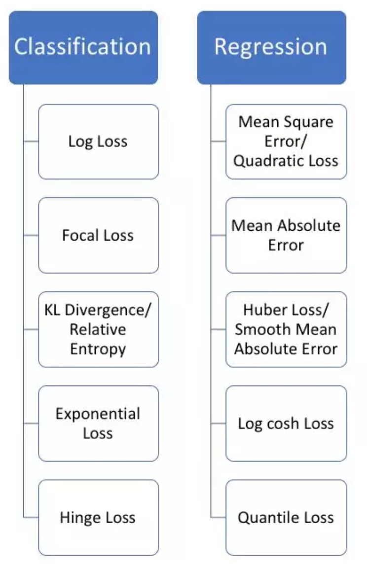
Less is More


  • 首页

  • 标签

  • 归档

  • 搜索

metrics

发表于 2020-10-09 |

分类指标

  • recall:召回率
  • precision:准确率
  • accuracy:正确率
  • F-Measure
  • sensitivity:灵敏度
  • specificity:特异度
  • TPR
  • FPR
  • ROC
  • AUC
  1. 混淆矩阵

    | | gt is p | gt is n |
    | :———-: | :————: | :—————: |
    | pred is p | tp | fp(假阳性) |
    | pred is n | fn(漏检) | tn |

    • 注意区分fp和fn
    • fp:被错误地划分为正例的个数,即实际为负例但被分类器划分为正例的实例数
    • fn:被错误地划分为负例的个数,即实际为正例但被分类器划分为负例的实例数
  2. recall

    • 衡量查全率
    • 对gt is p做统计
    • $recall = \frac{tp}{tp+fn}$
  3. precision

    • 衡量查准率
    • 对pred is p做统计
    • $precision = \frac{tp}{tp+fp}$
  4. accuracy

    • 对的除以所有
    • $accuracy = \frac{tp+tn}{p+n}$
  5. sensitivity

    • 衡量分类器对正例的识别能力
    • 对gt is p做统计
    • $sensitivity = \frac{tp}{p}=\frac{tp}{tp+fn}$
  6. specificity

    • 衡量分类器对负例的识别能力
    • 对gt is n做统计
    • $specificity =\frac{tn}{n}= \frac{tn}{fp+tn}$
  7. F-measure

    • 综合考虑P和R,是Precision和Recall加权调和平均
    • $F = \frac{(a^2+1)PR}{a^2*P+R}$
    • $F_1 = \frac{2PR}{P+R}$
  8. TPR

    • 将正例分对的概率
    • 对gt is t做统计
    • $TPR = \frac{tp}{tp+fn}$
  9. FPR

    • 将负例错分为正例的概率
    • 对gt is n做统计
    • $FPR = \frac{fp}{fp+tn}$
    • FPR = 1 - 特异度
  10. ROC

    • 每个点的横坐标是FPR,纵坐标是TPR
    • 描绘了分类器在TP(真正的正例)和FP(错误的正例)间的trade-off
    • 通过变化阈值,得到不同的分类统计结果,连接这些点就形成ROC curve
    • 曲线在对角线左上方,离得越远说明分类效果好
    • P/R和ROC是两个不同的评价指标和计算方式,一般情况下,检索用前者,分类、识别等用后者
  11. AUC

    • AUC的值就是处于ROC curve下方的那部分面积的大小
    • 通常,AUC的值介于0.5到1.0之间

metric learning系列

发表于 2020-09-25 |

参考:https://gombru.github.io/2019/04/03/ranking_loss/,博主实验下来觉得Triplet Loss outperforms Cross-Entropy Loss

综述

  1. metric learning

    • 常规的cls loss系列(CE、BCE、MSE)的目标是predict a label
  • metric loss系列的目标则是predict relative distances between inputs
    • 常用场景:人脸 & fine-grained
  1. relation between samples

    • first get the embedded representation
    • then compute the similarity score
      • binary (similar / dissimilar)
      • regression (euclidian distance)
  2. 大类:不管叫啥,主体上就两类,二元组和三元组

    • common target:拉近类内距离,拉大类间距离

    • pairs

      • anchor + sample
        • positive pairs:distance —> 0
        • negative pairs:disctance > a margin
    • triplets
      • anchor + pos sample + neg sample
      • target:(dissimilar distance - similar distance) —> a margin
  3. papers

    [siamese network] Signature Verification using a ‘Siamese’ Time Delay Neural Network:1993,lecun,孪生网络始祖,俩个子网络sharing weights,距离用的是cosine distance,loss直接优化距离,优化target是个定值cosine=1.0/-1.0

    [contrastive loss] Dimensionality Reduction by Learning an Invariant Mapping:2006,lecun,contrastive loss始祖,研究的是高维特征向量向低维映射的非线性层,距离用的是euclidean distance,loss优化的是squared distance,优化target是0和m,similar pairs仍旧会被推向一个定点,没有解决论文声称的uniform distribution

    [triplet-loss] Learning Fine-grained Image Similarity with Deep Ranking:2014,Google,用了三元组,提出了triplet-loss

    [facenet] FaceNet: A Unified Embedding for Face Recognition and Clustering:2015,Google,用来识别人脸,用了三元组和triplet-loss,squared euclidean distance,优化目标是同类和异类pair之间的相对距离,困难样本(semi-hard & hard)对收敛起作用(加速/local minima),triplet-loss考虑了类间的离散性,但没有考虑类内的紧凑性

    [center-loss] A Discriminative Feature Learning Approach for Deep Face Recognition:2016,也是用在人脸任务上,优化目标是类内的绝对距离,而不是建模相对关系,center-loss直接优化的是类间的间凑性,类间的离散性靠的是softmax loss

    [triplet-center-loss] Triplet-Center Loss for Multi-View 3D Object Retrieval:2018,东拼西凑水论文

    [Hinge-loss] SVM margin

    [circle-loss] Circle Loss: A Unified Perspective of Pair Similarity Optimization:2020CVPR,旷视,提出了cls loss和metric loss的统一形式$minimize(s_n - s_p+m)$,在此基础上提出circle loss作为优化目标$(\alpha_n s_n - \alpha_p s_p) = m$,在toy scenario下展示了分类边界和梯度的改善。

    ~~~~~~~~~~~~~~~~~~~~~~~~~~~~~~~~~~~~~~~~~~~~~~

    [Hierarchical Similarity] Learning Hierarchical Similarity Metrics:2012CVPR,

    [Hierarchical Triplet Loss] Deep Metric Learning with Hierarchical Triplet Loss:2018ECCV,

    • Hierarchical classicification应该单独做一个系列,tobeadded
  4. 一些待明确的问题

    • anchor怎么选:facenet中说明,每个mini-batch中每个类别必须都有
    • pairs怎么实现(困难的定义):facenet中说明,hard distance sample in mini-batch
    • hingeloss & SVM推导
    • 常规使用?结合cls loss和metric loss还是只用metric loss:cls loss和metric loss本质上是一样的,都是希望同类样本输出一样,不同类样本输出不一样,只不过前者具有概率意义,后者具有距离意义。上面列出来的只有center loss是要跟cls loss结合起来用的,因为他只针对类内,不足以推动整个模型。

Signature Verification using a ‘Siamese’ Time Delay Neural Network

  1. 动机
    • verification of written signatures
    • propose Siamese
      • two identical sub-networks
      • joined at their outputs
      • measure the distance
    • verification process
      • a stored feature vector
      • a chosen threshold
  2. 方法
    • network
      • two inputs:extracting features
      • two sub-networks:share the same weights
      • one output:cosine of the angle between two feature vectors
      • target
        • two real signatures:cosine=1.0
        • with one forgery:cosine=-0.9 and cosine=-1.0
      • dataset
        • 50% genuine:genuine pairs
        • 40% genuine:forgery pairs
        • 10% genuine:zero-effort pairs

Dimensionality Reduction by Learning an Invariant Mapping

  1. 动机

    • dimensionality reduction
    • propose Dimensionality Reduction by Learning an Invariant Mapping (DrLIM)
      • globally co- herent non-linear function
      • relies solely on neighbor- hood relationships
      • invariant to certain transformations of the inputs
  2. 论点

    • most existing dimensionality reduction techniques
      • they do not produce a function (or a mapping) from input to manifold
      • new points with unknown relationships with training samples cannot be processed
      • they tend to cluster points in output space
      • a uniform distribution in the outer manifolds is desirable
    • proposed DrLIM
      • globally coherent non-linear function
      • neighborhood relationships that are independent from any distance metric
      • invariant to complicated non-linear trnasformations
        • lighting changes
        • geometric distortions
      • can be used to map new samples
    • empoly contrastive loss
      • neighbors are pulled together
      • non-neighbors are pushed apart
    • energy based model
      • euclidean distance
      • approximates the “semantic similarity”of the inputs in input space
  3. 方法

    • contrastive loss

      • conventional loss sum over samples

      • contrastive loss sum over pairs $(X_1, X_2, Y)$

        • similar pairs:$Y=0$
        • dissimilar:$Y=1$
      • euclidean distance

        • $L = (1-Y)\sum L_s ||G_w(X_1)-G_w(X_2)||_2 + Y\sum L_d ||G_w(X_1)-G_w(X_2)||_2$

        • $L_s$ should results in low values for similar pairs

        • $L_d$ should results in high values for dissimilar pairs
        • exact form:$L(W,Y,X_1,X_2) = (1-Y)\frac{1}{2}(D^2) + (Y)\frac{1}{2} \{max(0,m-D)\}^2$

    • spring model analogy

      • similar partial loss相当于给弹簧施加了一个恒定的力,向中心点挤压
      • dissimilar partial loss只对圈内的点施力,推出圈外就不管了

FaceNet: A Unified Embedding for Face Recognition and Clustering

  1. 动机

    • face tasks

      • face verification: is this the same person
      • face recognition: who is the person
      • clustering: find common people among the faces
    • learn a mapping

      • compact Euclidean space
      • where the Euclidean distance directly correspond to face similarity

  2. 论点

    • traditionally training classification layer

      • generalizes well to new faces? indirectness

      • large dimension feature representation inefficiency

      • use siamese pairs

        • the loss encourages all faces of one identity to project onto a single point
    • this paper

      • employ triplet loss
        • target:separate the positive pair from the negative by a distance margin
        • allows the faces of one identity to live on a manifold
      • obtain face embedding
        • l2 norm
        • a fixed d-dims hypersphere
      • large dataset
        • to attain the appropriate invariances to pose, illumination, and other variational conditions
      • architecture

        • explore two different deep network

  3. 方法

    • input:三元组,consist of two matching face thumbnails and a non-matching one

    • ouput:特征描述,a compact 128-D embedding living on the fixed hypersphere $||f(x)||_2=1$

    • triple-loss

      • target:all anchor-pos distances are smaller than any anchor-neg distances with a least margin $\alpha$
      • $L = \sum_i^N [||f(x_i^a) - f(x_i^p)||_2^2 - ||f(x_i^a) - f(x_i^n)||_2^2 + \alpha]$
      • hard triplets
    • hard samples

      • $argmax_{x_i^p}||f(x_i^a) - f(x_i^p)||_2^2$
      • $argmin_{x_i^n}||f(x_i^a) - f(x_i^n)||_2^2$
      • infeasible to compute over the whole set:mislabelled and poorly imaged faces would dominate the hard positives and negatives
      • off-line:use recent checkpoint to compute on a subset
      • online:select in mini-batch
    • mini-batch:

      • 每个类别都必须有正样本
      • 负样本是randomly sampled
    • hard sample

      • use all anchor-positive pairs
      • selecting the hard negatives
        • hardest negatives can lead to bad local minima in early stage
        • 先pick semi-hard:$||f(x_i^a) - f(x_i^p)||_2^2 < ||f(x_i^a) - f(x_i^n)||_2^2$
    • network

      • 一种straight的网络,引入了1x1 conv先压缩通道
      • Inception models:20x fewer params,5x fewer FLOPS
    • metric

      • same/different是由a squared L2 distance决定
      • 因此测试结果是d的函数
      • 定义true accepts:圈内对的,$TA(d)=\{(i,j)\in P_{same}, with D(x_i,x_j)\leq d\}$
      • 定义false accepts:圈内错的,$FA(d)=\{(i,j)\in P_{diff}, with D(x_i,x_j)\leq d\}$

      • 定义validation rate:$VAL(d) = \frac{|TA(d)|}{|P_{same}|}$

      • 定义false accept rate:$FAR(d) = \frac{|FA(d)|}{|P_{diff}|}$

A Discriminative Feature Learning Approach for Deep Face Recognition

  1. 动机

    • enhance the discriminationative power of the deeply learned features
    • joint supervision
      • softmax loss
      • center loss
    • two key learning objectives
      • inter-class dispension
      • intra-class compactness
  2. 论点

    • face recognition task requirement
      • the learned features need to be not only separable but also discriminative
      • generalized enough for the new unseen samples
    • the softmax loss only encourage the separability of features
      • 对分类边界、类内类间分布没有直接约束
    • contrastive loss & triplet loss
      • training pairs or triplets dramatically grows
      • slow convergence and instability
    • we propose
      • learn a center
      • simultaneously update the center and optimize the distances
      • joint supervision
        • softmax loss forces the deep features of different classes staying apart
        • center loss efficiently pulls the deep features of the same class to their centers
        • to be more discriminationative
      • the inter-class features differences are enlarged
      • the intra-class features variations are reduced
  3. 方法

    • softmax vis

      • 最后一层hidden layer使用两个神经元
      • so that we can directly plot
      • separable but still show significant intra-class variations

    • center loss

      • $L_c = \frac{1}{2} \sum_1^m ||x_i - c_{y_i}||_2^2$

      • update class center on mini-batch:

      • joint supervision:

    • discussion

      • necessity of joint supervision
        • solely softmax loss —-> large intra-class variations
        • solely center loss —-> features and centers will degraded to zeros
      • compared to contrastive loss and triplet loss
        • using pairs:suffer from dramatic data expansion
        • hard mining:complex recombination
        • optimizing target:
          • center loss直接针对intra-class compactness,类内用距离来约束,类间用softmax来约束
          • contrastive loss也是直接优化绝对距离,类内&类间都用距离来约束
          • triplet loss是建模相对关系,类内&类间都用距离来约束
    • architecture

      • local convolution layer:当数据集在不同的区域有不同的特征分布时,适合用local-Conv,典型的例子就是人脸识别,一般人的面部都集中在图像的中央,因此我们希望当conv窗口滑过这块区域的时候,权重和其他边缘区域是不同的
      • 参数量暴增:kernel_size kernel_size output_size output_size input_channel * output_channel

  4. 实验

    • hyperparam:$\lambda$ and $\alpha$

      • fix $\alpha=0.5$ and vary $\lambda$ from 0-0.1
      • fix $\lambda=0.003$ and vary $\alpha$ from 0.01-1
      • 结论是remains stable across a large range,没有给出最佳/建议

    • 我的实验

      • 加比不加训练慢得多
      • 在Mnist上测试同样的epoch加比不加准确率低
      • 之所以Center Loss是针对人脸识别的Loss是有原因的,个人认为人脸的中心性更强一些,也就是说一个人的所有脸取平均值之后的人脸我们还是可以辨识是不是这个人,所以Center Loss才能发挥作用

Circle Loss: A Unified Perspective of Pair Similarity Optimization

  1. 动机

    • pair similarity
    • circular decision boundary
    • unify cls-based & metric-based data
      • class-level labels
      • pair-wise labels
  2. 论点

    • there is no intrinsic difference between softmax loss & metric loss

      • minimize between-class similarity $s_n$
      • maximize within- class similarity $s_p$
      • reduce $s_n - s_p$
    • short-commings

      • lack of flexibility:$s_p$和$s_n$的优化速度可能不同,一个快收敛了一个还很差,这时候用同样的梯度去更新就非常inefficient and irrational,就左图来说,下面的点相对上面的点,$s_n$更小(更接近op),$s_p$更小(更远离op),vice versa,但是决策平面对三个点相对于$s_n$和$s_p$的梯度都是一样的(1和-1)。
      • ambiguous convergence status:用一个hard distance margin来描述decision boundary还不够discriminative,hard decision boundary上各点其实还是有差别的,假设存在一个optimum($s_p=1 \ \& \ s_n=0$),那么左图决策平面上两个点,相对optimum的意义明显不一样,决策平面应该是个围绕optimum的圆圈。

    • propose circle loss

      • independent weighting factors:离optimum越远的penalty strength越大,这一项直接以距离为优化目标的loss都是满足的
      • different penalty strength:$s_p$和$s_n$ learn at different paces,类内加权,加权系数是learnable params
      • $(\alpha_n s_n - \alpha_p s_p) = m$:yielding a circle shape
  3. 方法

    • 核心:$(\alpha_n s_n - \alpha_p s_p) = m$

    • self-paced weighting

      • given optimum $O_p$ and $O_n$,for each similarity score:

      • cut-off at zero

      • 对于远离optimum的点梯度放大,接近optimum的点(快收敛)梯度缩小

      • softmax里面通常不会对同类样本间做这种rescaling的,因为它希望所有样本value都达到贼大

      • Circle loss abandons the interpretation of classifying a sample to its target class with a large probability

    • margin

      • adding a margin m reinforces the optimization
      • take toy scenario
        • 最终整理成:$(s_n-0)^2 + (s_p-1)^2 = 2m^2$
        • op target:$s_p > 1-m$,$s_n < m$
        • relaxation factor $m$:controls the radius of the decision boundary
    • unified perspective

      • tranverse all the similarity pairs:$\{s_p^i\}^K$和$\{s_n^j\}^N$
      • to reduce $(s_n^j - s_p^i)$:$L_{uni}=log[1+\sum^K_i \sum^N_j exp(\lambda (s_n^j - s_p^i + m))]$
      • 解耦(不会同时是$s_p$和$s_n$):$L_{uni}=log[1+\sum^N_j exp(\lambda (s_n^j + m))\sum^K_i exp(\lambda (-s_p^i))]$
      • given class labels:
        • we get $(N-1)$ between-class similarity scores and $(1)$ within-class similarity score
        • 分母翻上去:$L = -log \frac{exp(\lambda (s_p-m))}{exp(\lambda (s_p-m)) + \sum^{N-1}_j exp(\lambda (s_n^j))}$
        • 就是softmax
      • given pair-wise labels:
        • triplet loss with hard mining:find pairs with large $s_n$ and low $s_p$
        • use infinite:$L=lim_{\lambda \to \inf} \frac{1}{\lambda} L_{uni}$
  4. 实验

    • Face recognition
      • noisy and long-tailed data:去噪并且去掉稀疏样本
      • resnet & 512-d feature embeddings & cosine distance
      • $\lambda=256$,$m=0.25$
    • Person re-identification
      • $\lambda=128$,$m=0.25$
    • Fine-grained image retrieval
      • 车集和鸟集
      • bn-inception & 512-d embeddings
      • P-K sampling
      • $\lambda=80$,$m=0.4$
    • hyper-params
      • the scale factor $\lambda$:
        • determines the largest scale of each similarity score
        • Circle loss exhibits high robustness on $\lambda$
        • the other two becomes unstable with larger $\lambda$
        • owing to the decay factor
      • the relaxation factor m:
        • determines the radius of the circular decision boundary
        • surpasses the best performance of the other two in full range
        • robustness
  5. inference

    • 对人脸类任务,通常用训练好的模型生成一个人脸标准底库,然后每次推理的时候得到测试数据的特征向量,并在标准底库中搜索相似度最高的特征,完成人脸识别过程。

efficient周边

发表于 2020-09-23 |

因为不是googlenet家族官方出品,所以放在外面

[EfficientFCN] EfficientFCN: Holistically-guided Decoding for Semantic Segmentation:商汤,主要针对upsampling是局部感受野,重建失真多,分割精度差的问题,提出了Holistically-guided Decoder (HGD) ,用来recover the high-resolution (OS=8) feature maps,想法上接近SCSE-block,数学表达上接近bilinear-CNN,性能提升主要归因于eff back吧。

EfficientFCN: Holistically-guided Decoding for Semantic Segmentation

  1. 动机

    • Semantic Segmentation
      • dilatedFCN:computational complexity
      • encoder-decoder:performance
    • proposed EfficientFCN
      • common back without dilated convolution
      • holistically-guided decoder
    • balance performance and efficiency
  2. 论点

    • key elements for semantic segmentation
      • high-resolution feature maps
      • pre-trained weights
    • OS32 feature map:the fine-grained structural information is discarded
    • dilated convolution:no extra parameters introduced but equire high computational complexity and memory consumption
    • encoder-decoder based methods
      • repeated upsampling + skip connection procedure
        • upsampling
        • concat/add
        • successive convs
      • Even with the skip connections, lower-level high-resolution feature maps cannot provide abstractive enough features for achieving high- performance segmentation
      • The bilinear upsampling or deconvolution operations are conducted in a local manner(from a limited receptive filed)
      • improvements
        • reweight:SE-block
        • scales each feature channel but maintains the original spatial size and structures:【scse block对spacial有加权啊】
    • propose EfficientFCN

      • widely used classification model
      • Holistically-guided Decoder (HGD)
        • take OS8, OS16, OS32 feature maps from backbone
        • OS8和OS16用来spatially guiding the feature upsampling process
        • OS32用来encode the global context然后基于guidance进行上采样
        • linear assembly at each high-resolution spatial location:感觉就是对上采样特征图做了加权

  3. 方法

    • Holistically-guided Decoder

      • multi-scale feature fusion
      • holistic codebook generation
        • from high-level feature maps
        • holistic codewords:without any spatial order
      • codeword assembly

    • multi-scale feature fusion

      • we observe the fusion of multi-scale feature maps generally result in better performance
      • compress:separate 1x1 convs
      • bilinear downsamp/upsamp
      • concatenate
      • fused OS32 $m_{32}$ & fused OS8 $m_8$
    • holistic codebook generation

      • from $m_{32}$
      • two separate 1x1 conv
        • a codeword based map $B \in R^{1024(H/32)(W/32)}$:每个位置用一个1024-dim的vector来描述
        • n spatial weighting map $A\in R^{n(H/32)(W/32)}$:highlight 特征图上不同区域
          • softmax norm in spatial-dim
          • $\widetilde A_i(x,y)=\frac{exp(A_i(x,y))}{\sum_{p,q} exp(A_i(p,q))}, i\in [0,n)$
      • codeword $c_i \in R^{1024}$
        • global description for each weighting map
        • weighted average of B on all locations
        • $c_i = \sum_{p,q} \widetilde A_i(p,q) B(p,q)$
        • each codeword captures certain aspect of the global context
      • orderless high-level global features $C \in R^{1024*n}$
        • $C = [c_1, …, c_n]$
    • codeword assembly

      • raw guidance map $G \in R^{1024(H/8)(W/8)}$:1x1 conv on $m_8$
      • fuse semantic-rich feature map $\overline B \in R^{1024}$:global average vector
      • novel guidance feature map $\overline G = G \oplus \overline B $:location-wise addition【????】
      • linear assembly weights of the n codewords $W \in R^{n(H/8)(W/8)}$:1x1 conv on $\overline G$
      • holistically-guided upsampled feature $\tilde f_8 = W^T C$:reshape & dot
      • final feature map $f_8$:concat $\tilde f_8$ and $G$
    • final segmentation

      • 1x1 conv
      • further upsampling
  4. 实验

    • numer of holistic codewords

      • 32-512:increase
      • 512-1024:slight drop
      • we observe the number of codewords needed is approximately 4 times than the number of classes

data aug

发表于 2020-09-18 |

[mixup] mixup: BEYOND EMPIRICAL RISK MINIMIZATION:对不同类别的样本,不仅可以作为数据增广手段,还可以用于semi-supervised learning(MixMatch)

[mixmatch] MixMatch: A Holistic Approach to Semi-Supervised Learning:针对半监督数据的数据增广

[mosaic] from YOLOv4

[AutoAugment] AutoAugment: Learning Augmentation Policies from Data:google

[RandAugment] RandAugment: Practical automated data augmentation with a reduced search space:google

RandAugment: Practical automated data augmentation with a reduced search space

  1. 动机

    • AutoAugment
      • separate search phase
      • run on a subset of a huge dataset
      • unable to adjust the regularization strength based on model or dataset size
    • RandAugment

      • significantly reduced search space
      • can be used uniformly across tasks and datasets
      • match or exceeds the previous val acc

  2. 方法

    • formulation

      • always select a transformation with uniform prob $\frac{1}{K}$

      • given N transformations for an image:there are $K^N$ potential policies

      • fixied magnitude schedule M:we choose Constant,因为只要一个hyper

      • run naive grid search

    • 疑问:这样每个op等概率,就不再data-specific了,也看不出自然图像更prefer color transformation这种结论了

AutoAugment: Learning Augmentation Policies from Data

  1. 动机

    • search for data augmentation policies

    • propose AutoAugment

      • create a search space composed of augmentation sub-policies
        • one sub-policy is randomly choosed per image per mini-batch
        • a sub-policy consists of two base operations
      • find the best policy:yields the highest val acc on the target dataset

      • the learned policy can transfer

  2. 论点

    • data augmentation
      • to teach a model about invariance
      • in data domain is easier than hardcoding it into model architecture
      • currently dataset-specific and often do not transfer:
        • MNIST:elastic distortions, scale, translation, and rotation
        • CIFAR & ImageNet:random cropping, image mirroring and color shifting / whitening
        • GAN:直接生成图像,没有归纳policy
    • we aim to automate the process of finding an effective data augmentation policy for a target dataset
      • each policy:
        • operations in certain order
        • probabilities after applying
        • magnitudes
      • use reinforcement learning as the search algorithm
    • contributions
      • SOTA on CIFAR & ImageNet & SVHN
      • new insight on transfer learning:使用预训练权重没有显著提升的dataset上,使用同样的aug policies则会涨点
  3. 方法

    • formulation

      • search space of policies

        • policy:a policy consists of 5 sub-policies
        • sub-policy:each sub-policy consisting of two image operations
        • operation:each operation is also associated with two hyperparameters
          • probability:of applying the operation,uniformly discrete into 11 values
          • magnitude:of the operation,uniformly discrete into 10 values
        • a mini-batch share the same chosen sub-policy
      • operations:16 in total,mainly use PIL

        • https://blog.csdn.net/u011583927/article/details/104724419有各种operation的可视化效果
        • shear是砍掉图像一个角的畸变
        • equalize是直方图均衡化
        • solarize是基于一定阈值的invert,高于阈值invert,低于阈值不变
        • posterize也是一种像素值截断操作
        • color是调整饱和度,mag<1趋近灰度图
        • sharpness决定图像模糊/锐化
        • sample pairing:两张图加权求和,但是不改变标签
      • searching goal

        • with $(161011)^2$ choices of sub-policies
        • we want 5
    • example

      • 一个sub-policy包含两个operation
      • 每个operation有一定的possibility做/不做
      • 每个operation有一定的magnitude决定做后的效果

  4. 结论

    • On CIFAR-10, AutoAugment picks mostly color-based transformations

    • on ImageNet, AutoAugment focus on color-based transformations as well, besides geometric transformation and rotate is commonly used

      • one of the best policy

      • overall results

mixup: BEYOND EMPIRICAL RISK MINIMIZATION

  1. 动机

    • classification task
    • memorization and sensitivity issue
      • reduces the memorization of corrupt labels
      • increases the robustness to adversarial examples
      • improves the generalization
      • can be used to stabilize the training of GANs
    • propose convex combinations of pairs of examples and their labels
  2. 论点

    • ERM(Empirical Risk Minimization):issue of generalization

      • allows large neural networks to memorize (instead of generalize from) the training data even in the presence of strong regularization
      • neural networks change their predictions drastically when evaluated on examples just outside the training distribution
    • VRM(Vicinal Risk Minimization):introduce data augmentation

      • e.g. define the vicinity of one image as the set of its horizontal reflections, slight rotations, and mild scalings
      • vicinity share the same class
      • does not model the vicinity relation across examples of different classes
    • ERM中的training set并不是数据的真实分布,只是用有限数据来近似真实分布,memorization也会最小化training error,但是对training seg以外的sample就leads to undesirable behaviour
    • mixup就是VRM的一种,propose a generic vicinal distribution,补充vicinity relation across examples of different classes
  3. 方法

    • mixup

      • constructs virtual training examples

      • use two examples drawn at random:raw inputs & raw one-hot labels

      • 理论基础:linear interpolations of feature vectors should lead to linear interpolations of the associated targets

      • hyper-parameter $\alpha$

        • $\lambda = np.random.beta(\alpha, \alpha)$
      • controls the strength of interpolation
    • 初步结论

    • three or more examples mixup does not provide further gain but more computation

    • interpolating only between inputs with equal label did not lead to the performance gains

    • key elemets——two inputs with different label

    • vis

      • decision boundaries有了一个线性过渡

      • 更准确 & 梯度更小:error少所以loss小所以梯度小??

  4. 实验

    • 初步分类实验

      • $\alpha \in [0.1, 0.4]$ leads to improved performance,largers leads to underfitting
      • models with higher capacities and/or longer training runs are the ones to benefit the most from mixup
    • memorization of corrupted labels

      • 将数据集中一部分label换成random noise
      • ERM直接过拟合,在corrupted sample上面training error最小,测试集上test error最大
      • dropout有效防止过拟合,但是mixup outperforms它
      • corrupted label多的情况下,dropout+mixup performs the best

    • robustness to adversarial examples

      • Adversarial examples are obtained by adding tiny (visually imperceptible) perturbations
      • 常规操作data augmentation:produce and train on adversarial examples
      • add significant computational:样本数量增多,梯度变化大
      • mixup results in a smaller loss and gradient norm:因为mixup生成的假样本“更合理一点”,梯度变化更小
    • ablation study

      • mixup is the best:绝对领先第二mix input + label smoothing

      • the effect of regularization

        • ERM需要大weight decay,mixup需要小的——说明mixup本身的regularization effects更强
        • 高层特征mixup需要更大的weight decay——随着层数加深regularization effects减弱
        • AC+RP最强

        • label smoothing和add Gaussian noise to inputs 相对比较弱

        • mix inputs only(SMOTE) shows no gain

MixMatch: A Holistic Approach to Semi-Supervised Learning

  1. 动机

    • semi-supervised learning
    • unify previous methods
    • proposed mixmatch
      • guessing low-entropy labels
      • mixup labeled and unlabeled data
    • useful for differentially private learning
  2. 论点

    • semi-supervised learning add a loss term computed on unlabeled data and encourages the model to generalize better to unseen data
    • the loss term
      • entropy minimization:decision boundary应该尽可能远离数据簇,因此prediction on unlabeled data也应该是high confidence
      • consistency regularization:增强前后的unlabeled data输出分布一致
      • generic regularization:weight decay & mixup
    • MixMatch unified all above
      • introduces a unified loss term for unlabeled data
  3. 方法

    • overview

      • given:a batch of labeled examples $X$ and a batch of labeled examples $U$
      • augment+label guess:a batch of augmented labeled examples $X^{‘}$ and a batch of augmented labeled examples $U^{‘}$
      • compute:separate labeled and unlabeled loss terms $L_X$ and $L_U$
      • combine:weighted sum

    • MixMatch

      • data augmentation

        • 常规augmentation
        • 作用于每一个$x_b$和$u_b$
        • $u_b$做$K$次增强
      • label guessing

        • 对增强的$K$个$u_b$分别预测,然后取平均
        • average class prediction
      • sharpening

        • reduce the entropy of the label distribution
        • 拉高最大prediction,拉小其他的
        • $Sharpen (p, T)_i =\frac{p_i^{\frac{1}{T}}}{\sum^{N}_j p_j^{\frac{1}{T}}} $
        • $T$趋近于0的时候,processed label就接近one-hot了
      • mixup

        • slightly modified form of mixup to make the generated sample being more closer to the original

      • loss function

        • labeled loss:typical cross-entropy loss
      • unlabeled loss:squared L2,bounded and less sensitive to completely incorrect predictions

    • hyperparameters

      • sharpening temperature $T$:fixed 0.5

        • number of unlabeled augmentations $K$:fixed 2
        • MixUp Beta parameter $\alpha$:0.75 for start
        • unsupervised loss weight $\lambda_U$:100 for start
      • Algorithm

  4. 实验

[mosaic] from YOLOv4

hrnet

发表于 2020-09-18 |

papers

  • [v1 2019] Deep High-Resolution Representation Learning for Human Pose Estimation:base HRNet,提出parallel multi-resolution subnetworks,highest resolution output作为输出
  • [v2 2019] High-Resolution Representations for Labeling Pixels and Regions:simple modification,在末端输出的时候加了一步融合,将所有resolution-level的feature上采样到output-level然后concat

Deep High-Resolution Representation Learning for Human Pose Estimation

  1. 动机

    • human pose estimation
    • high-resolution representations through
      • existing methods recover high-res feature from the low,大多数方法是recover系
      • this methods maintain the high-res from start to the end,本文是maintaining系
      • add high-to-low resolution subnetworks
      • repeated multi-scale fusions
    • more accurate and spatially more precise
    • estimate on the high-res output,最后的high-res representation作为输出,接各种task heads
  2. 论点

    • in parallel rather than in series:potentially spatially more precise,相比较于recover类的架构,不会导致过多的spatial resolution loss,recover类的架构有时会用空洞卷积来维持resolution来降低spatial resolution loss

    • repeated multi- scale fusions:boost both high&low representations,more accurate

    • pose estimation

      • probabilistic graphical model
      • regression
      • heatmap
    • High-to-low and low-to-high frameworks

      • Symmetric high-to-low and low-to-high:Hourglass
      • Heavy high-to-low and light low-to-high:ResNet back + simple bilinear upsampling
      • Heavy high-to-low with dilated convolutions and further lighter low-to-high:ResNet with atrous conv + fewer bilinear upsampling

      • high-to-low part和low-to-hight part:有对称和不对称两种,对称就如Hourglass,不对称就是down-path使用heavy classification backboens,up-path使用轻量的上采样

      • fusion:
        • a和b都有skip-connections,将down-path和up-path的特征融合,目的是融合low-level和high-level的特征
        • a里面还有不同resolution level的融合
        • fusion方式有sum/concat
      • refinenet:也就是up-path,可以用upSampling/transpose convs
  3. 方法

    • task description

      • human pose estimation = keypoint detection
      • detect K keypoints from an Image (H,W,3)
      • state-of-the art methods:predict K heatmaps,each indicates one of the keypoint
        • a stem with 2 strided conv
        • a body outputting features with the same input resolution
        • a regressor estimating heatmaps
      • we focus on the design of the main body
    • sequential & parallel multi-resolution networks

      • notation:$N_{sr}$

        • s is the stage
        • r is the resolution index,denotes $\frac{1}{2^{r-1}}$ of the resolution of the first subnetwork
      • sequential

      • parallel

    • overview

      • four stages
      • channels double when halve the res
      • 1st stage
        • 第一个stage是一个high-resolution subnetwork,没有下采样,没有parallel分支
        • 4 residual units,bottleneck resblock
        • width=64
        • 3x3 conv reducing width to C
      • 2、3、4 stages
        • 接下来的stage gradually add high-to-low subnetwork
        • 是multi-resolution subnetworks
        • 每个subnetwork都比前一个多一个extra lower one resolution
        • contain 1, 4, 3 exchange blocks respectively
        • exchange block
          • conv:4 residual units,two 3x3 conv
          • exchange unit
      • width
        • C:width of the high-resolution subnetworks in last three stages
        • other three parallel subnetworks
          • HRNet-W32:64, 128, 256
          • HRNet-W48:96, 192, 384
    • repeated multi-scale fusion

      • exchange blocks:每个high-to-low subnetwork包含多个parallel分支,每条path称为exchange block,每个exchange block包含一系列3-conv-units + a exchange unit

      • 3-conv-units:堆叠卷积核,提取特征,加深网络

      • exchange unit:交换不同resolution level的信息

        • notations:一系列输入$\{X_1,X_2, …, X_r\}$,一系列输出$\{Y_1,Y_2, …, Y_r\}$,如果跨stage还有一个$Y_{r+1}$

        • 每个$Y_k$都是一个aggregation of the input maps:$Y_k=\sum^s_i a(X_i,k)$

          • i<k:需要下采样,每下采样一倍都是一个stride2-3x3-conv
          • i=k:identify connection
          • i>k:需要上采样,nearest neighbor upsamp + 1x1-align-conv
          • k=$r+1$:需要在$Y_r$的基础上,在执行一次stride2-3x3-conv下采样得到

      • fusion:sum,所以上/下采样都需要通道对齐,输出map和对应level的输入map保持尺寸不变

    • heatmap estimation

      • from the last high-res exchange unit
      • mse
      • gt gassian map:std=1
    • network instantiation

      • stem + 4 stages
      • 每个new stage input:res halved and channel doubled
      • stem
        • 两个s2-conv-bn-relu,channel 64
      • first stage:
        • 使用和ResNet-50中一样的4个residual units,channel 64
        • 然后用一个3x3-conv调整channel到一个起始channel C
      • 2/3/4 stage
        • 堆叠exchange blocks,分别有1/4/3个exchange block
        • 每个exchange block使用4个residual units和1个exchange unit
        • 也就是总共有8次multi-scale fusion
        • channel C/2C/4C
      • HRNet-32:C=64
      • HRNet-48:C=96

HRNet v2: High-Resolution Representations for Labeling Pixels and Regions

  1. 动机

    • High-resolution representation很重要
    • HRNet v1已经有不错的结果
    • a further study on high resolution representations
    • a small modification:之前只关注high-resolution representations,现在关注所有level的output representations
  2. 论点

    • 获得high resolution representation的两大方式

      • recover系:先下采样,然后用low-resolution重建,Hourglass,U-net,encoder-decoder
      • maintain系:始终保留high-resolution的representation,同时不断用parallel low-resolution representations来strengthen,HRNet
    • HRNet

      • maintains high-resolution representations
      • connecting high-to-low resolution convolutions in parallel
      • repeatedly conducting multi-scale fusions across levels
      • 简单来说,就是在每个阶段,保留现有resolution level,同时
      • 不仅representation足够强大(融合了low-level high semantic info),还spatially precise

    • our modification HRNetV2

      • HRNet 里面我们只关注最上面的high-resolution representation
      • HRNet V2里面我们探索所有high-to-low parallel paths上面的representations
      • 在语意分割任务中我们使用output high resolution representations来生成heatmaps
      • 在检测任务中我们将multi-level的representations给到FastRCNN
  3. 方法

    • Architecture

      • multi-resolution block
        • multi-resolution group convolution:在每个representation level分别执行分组卷积,deeper
        • multi-resolution convolution:发生在所有representation level上
        • 下采样:stride-2 3x3 conv
        • 上采样:bilinear /nearest neighbor
    • Modification

      • HRNetV1:只把最后一个阶段 highest resolution的representation作为输出
      • HRNetV2:最后一个阶段,每个resolution level的representations都上采样到highest,然后concat作为输出,甚至还将这个输出进一步下采样得到feature pyramid

      • HRNet for classification:也可以反向操作,将最后一个阶段每个resolution level的representations都下采样到lowest,然后sum,最后output 2048-dim representation is fed into the classifier

  4. 实验

bilinear CNN

发表于 2020-09-18 |

17年的paper,引用量15,提出了网路结构,但是没分析为啥有效,垃圾

Bilinear CNNs for Fine-grained Visual Recognition

  1. 动机

    • fine-grained classification
    • propose a pooled outer product of features derived from two CNNs
      • 2 CNNs
      • a bilinear layer
      • a pooling layer
    • outperform existing models and fairly efficient
    • effective at other image classification tasks such as material, texture, and scene recognition
  2. 论点

    • fine-grained classification tasks require
      • recognition of highly localized attributes of objects
      • while being invariant to their pose and location in the image
    • previous techniques
      • part-based models
        • construct representations by localizing parts
        • more accurate but requires part annotations
      • holistic models
        • construct a representation of the entire image
        • texture descriptors:FV,SIFT
      • STN:augment CNNs with parameterized image transformations
      • attention:use segmentation as a weakly-supervised manner
    • Our key insight is that several widely-used texture representations can be written as a pooled outer product of two suitably designed features
      • several widely-used texture representations
      • two suitably designed features
    • the bilinear features are highly redundant
      • dimensionality reduction
      • trade-off between accuracy
    • We also found that feature normalization and domain-specific fine-tuning offers additional benefits

    • combination

      • concatenate:additional parameters to fuse
      • an outer product:no parameters
      • sum product:can achieve similar approximations
    • “two-stream” architectures
      • one used to model two- factor variations such as “style” and “content” for images
      • in our case is to model two factor variations in location and appearance of parts:但并不是explicit modeling因为最终是个分类头
      • one used to analyze videos modeling the temporal aspect and the spatial aspect
    • dimension reduction
      • two 512-dim feature results in 512x512-dim
      • earlier work projects one feature to a lower-dimensional space, e.g. 64-dim—>512x64-dim
      • we use compact bilinear pooling to generate low-dimensional embeddings (8-32x)
  3. 方法

    • architecture

      • input $(l,I)$:takes an image and a location,location generally contains position and scale
      • quadruple $B=(f_A, f_B, P, C)$
      • A、B两个CNN:conv+pooling layers,
      • P:pooling function
        • combined A&B outputs using the matrix outer product
        • average pooling
      • C:logistic regression or linear SVM
        • we found that linear models are effective on top of bilinear features
    • CNN

      • independent/partial shared/fully shared

    • bilinear combination

      • for each location

      • $bilinear(l,I,f_A,f_B)=f_A(l,I)^T f_B(l,I)$

      • pooling function combines bilinear features across all locations

      • $\Phi (I) = \sum_{l\in L} bilinear(l,I,f_A,f_B)$

      • same feature dimension K for A & B,e.g. KxM & KxN respectively,$\Phi(I)$ is size MxN

      • Normalization

        • a signed square root:$y=sign(x)\sqrt {|x|}$
        • follow a l2 norm:$z = \frac{y}{||y||_2}$

        • improves performance in practice

    • classification

      • logistic regression or linear SVM
      • we found that linear models are effective on top of bilinear features
    • back propagation

      • $\frac{dl}{dA}=B(\frac{dl}{dx})^T$,$\frac{dl}{dB}=A(\frac{dl}{dx})^T$

    • Relation to classical texture representations:放在这一节撑篇幅??

      • texture representations can be defined by the choice of the local features, the encoding function, the pooling function, and the normalization function
        • choice of local features:orderless aggregation with sum/max operation
        • encoding function:A non-linear encoding is typically applied to the local feature before aggregation
        • normalization:normalization of the aggregated feature is done to increase invariance
      • end-to-end trainable

label smoothing

发表于 2020-09-14 |
  1. 动机

    • to understand label smoothing
      • improving generalization
      • improves model calibration
      • changes the representations learned by the penultimate layer of the network
      • effect on knowledge distillation of a student network
    • soft targets:a hard target and the uniform distribution of other classes
  2. 论点

    • label smoothing implicitly calibrates the learned models
      • 能让confidences更有解释性——more aligned with the accuracies of their predictions
      • label smoothing impairs distillation——teacher用了label smoothing,student会表现变差,this adverse effect results from loss of information in the digits
  3. 方法

    • modeling

      • penultimate layer:fc with activation
        • $p_k = \frac{e^{wx}}{\sum e^{wx}}$
      • outputs:loss
        • $H(y,p)=\sum_{k=1}^K -y_klog(p_k)$
      • hard targets:$y_k$ is 1 for the correct class and 0 for the rest
      • label smoothing:$y_k^{LS} = y_k(1-\alpha)+ \alpha /K$
    • visualization schem

      • 将dimK activation vector投影到正交平面上,a dim2 vector per example
      • clusters are much tighter because label smoothing encourages that each example in training set to be equidistant from all the other class’s templates

      • 3 classes shows triangle structure since ‘equidistant’

      • predictions‘ absolute values are much bigger without LM, representing over-confident
      • semantically similar classes are harder to separate,但是总体上cluster形态还是好一点
      • training without label smoothing there is continuous degree of change between two semantically similar classes,用了LM以后就观察不到了——相似class之间的语义相关性被破坏了,’erasure of information’
      • have similar accuracies despite qualitatively different clustering,对分类精度的提升不明显,但是从cluster形态上看更好看
    • model calibration

      • making the confidence of its predictions more accurately represent their accuracy

      • metric:expected calibration error (ECE)

      • reliability diagram

      • better calibration compared to the unscaled network

      • Despite trying to collapse the training examples to tiny clusters, these networks generalize and are calibrated:在训练集上的cluster分布非常紧凑,encourage每个样本都和其他类别的cluster保持相同的距离,但是在测试集上,样本的分布就比较松散了,不会限定在小小的一坨内,说明网络没有over-confident,representing the full range of confidences for each prediction

    • knowledge distillation

      • even when label smoothing improves the accuracy of the teacher network, teachers trained with label smoothing produce inferior student networks

      • As the representations collapse to small clusters of points, much of the information that could have helped distinguish examples is lost

      • 看training set的scatter,LM会倾向于将一类sample集中成为相似的表征,sample之间的差异性信息丢了:Therefore a teacher with better accuracy is not necessarily the one that distills better

noisy student

发表于 2020-09-11 |

Self-training with Noisy Student improves ImageNet classification

  1. 动机

    • semi-supervised learning(SSL)
    • semi-supervised approach when labeled data is abundant
    • use unlabeled images to improve SOTA model
    • improve self-training and distillation
    • accuracy and robustness
    • better acc, mCE, mFR
      • EfficientNet model on labeled images
    • student
      • even or larger student model
      • on labeled & pseudo labeled images
      • noise, stochastic depth, data augmentation
      • generalizes better
    • process iteration
      • by putting back the student as the teacher
  2. 论点

    • supervised learning which requires a large corpus of labeled images to work well
    • robustness
      • noisy data:unlabeled images that do not belong to any category in ImageNet
      • large margins on much harder test sets
    • training process
      • teacher
        • EfficientNet model on labeled images
      • student
        • even or larger student model
        • on labeled & pseudo labeled images
        • noise, stochastic depth, data augmentation
        • generalizes better
      • process iteration
        • by putting back the student as the teacher
    • improve in two ways
      • it makes the student larger:因为用了更多数据
      • noised student is forced to learn harder:因为label有pseudo labels,input有各类augmentation,网络有dropout/stochastic depth
    • main difference compared with Knowledge Distillation
      • use noise ——— KD do not use
      • use equal/larger student ——— KD use smaller student to learn faster
    • think of as Knowledge Expansion
      • giving the student model enough capacity and difficult environments
      • want the student to be better than the teacher
  3. 方法

    • algorithm
      • train teacher use labeled images
      • use teacher to inference unlabedled images, generating pseudo labels, soft/one-hot
      • train student model use labeled & unlabeld images
      • make student the new teacher, jump to the inter step
    • noise
      • enforcing invariances:要求student网络能够对各种增强后的数据预测label一样,ensure consistency
      • required to mimic a more powerful ensemble model:teacher网络在inference阶段进行dropout和stochastic depth,behaves like an ensemble,whereas the student behaves like a single model,这就push student网络去学习一个更强大的模型
    • other techniques
      • data filtering
        • we filter images that the teacher model has low confidences
        • 这部分data与training data的分布范围内
      • data balancing
        • duplicate images in classes where there are not enough images
        • take the images with the highest confidence when there are too many
    • soft/hard pseudo labels
      • both work
      • soft slightly better
  4. 实验

    • dataset
      • benchmarked dataset:ImageNet 2012 ILSVRC
      • unlabeled dataset:JFT
      • fillter & balancing:
        • use EfficientNet-B0
        • trained on ImageNet,inference over JFT
        • take images with confidence over 0.3
        • 130M at most per class
    • models
      • EfficientNet-L2
        • further scale up EfficientNet-B7
        • wider & deeper
        • lower resolution
        • train-test resolution discrepancy
          • first perform normal training with a smaller resolution for 350 epochs
          • then finetune the model with a larger resolution for 1.5 epochs on unaugmented labeled images
          • shallow layers are fixed during finetuning
      • noise
        • stochastic depth:stochastic depth 0.8 for the final layer and follow the linear decay rule for other layers
        • dropout:dropout 0.5 for the final layer
        • RandAugment:two random operations with magnitude set to 27
    • iterative training

      • 【teacher】first trained an EfficientNet-B7 on ImageNet
      • 【student】then trained an EfficientNet-L2 with the unlabeled batch size set to 14 times the labeled batch size
      • 【new teacher】trained a new EfficientNet-L2
      • 【new student】trained an EfficientNet-L2 with the unlabeled batch size set to 28 times the labeled batch size
      • 【iteration】…
    • robustness test

      • difficult images
      • common corruptions and perturbations

      • FGSM attack

      • metrics

        • improves the top-1 accuracy
        • reduces mean corruption error (mCE)

        • reduces mean flip rate (mFR)

    • ablation study

      • noisy
        • 如果不noise the student,当student model的预测和teacher预测的unlabeled数据完全一样的情况下,loss为0,不再学习,这样student就不能outperform teacher了
        • injecting noise to the student model enables the teacher and the student to make different predictions
        • The student performance consistently drops with noise function removed
        • removing noise leads to a smaller drop in training loss,说明noise的作用不是为了preventing overfitting,就是为了enhance model
      • iteration
        • iterative training is effective in producing increas- ingly better models
        • larger batch size ratio for latter iteration

complement cross entropy

发表于 2020-09-08 |
  1. summary
    • 使用complement loss的主要动机是one-hot的label下,ce只关注拉高正样本概率,丧失掉了其他incorrect类别的信息
    • 事实上对于incorrect类别,可以让其输出概率值分布的熵尽可能的大——也就是将这个分布尽可能推向均匀分布,让它们之间互相遏制从而凸显出ground truth的概率
    • 但这是建立在“各个标签之间相互独立”这个假设上,如果类别间有hierarchical的关系/multi-label,就不行了。
    • 在数学表达上,
      • 首先仍然是用ce作用于correct label,希望正样本概率gt_pred尽可能提高,接近真实值
      • 然后是作用于incorrect label的cce,在除了正例pred possibility以外的几个概率上,计算交叉熵,希望这几个概率尽可能服从均匀分布,概率接近$\frac{1-gt_pred}{K-1}$
      • 我感觉这就是label smoothing,主要区别就是cce上有个norm项,label smoothin在计算ce的时候,vector中每一个incorrect label的熵都与correct label等权重,cce对整个incorrect vector的权重与correct label等同,且可以调整。

Imbalanced Image Classification with Complement Cross Entropy

  1. 动机

    • class-balanced datasets
    • motivated by COT(complement objective training)
      • suppressing softmax probabilities on incorrect classes during training
    • propose cce
      • keep ground truth probability overwhelm the other classes
      • neutralizing predicted probabilities on incorrect classes
  2. 论点

    • class imbalace
      • limits generalization
      • resample
        • oversampling on minority classes
        • undersampling on majority classes
      • reweight
        • neglect the fact that samples on minority classes may have noise or false annotations
        • might cause poor generalization
    • observed degradation in imbalanced datasets using CE
      • cross entropy mostly ignores output scores on wrong classes
      • neutralizing predicted probabilities on incorrect classes helps improve accuracy of prediction for imbalanced image classification
  3. 方法

    • complement entropy

      • calculated on incorrect classes
      • N samples,K-dims class vector
      • $C(y,\hat y)=-\frac{1}{N}\sum_{i=1}^N\sum_{j=1,j \neq g}^K \frac{\hat y^j}{1-\hat y^g}log\frac{\hat y^j}{1-\hat y^g} $
      • the purpose is to encourage larger gap between ground truth and other classes —— when the incorrect classes obey normal distribution it reaches optimal
    • balanced complement entropy

      • add balancing factor
      • $C^{‘}(y,\hat y) = \frac{1}{K-1}C(y,\hat y)$
    • forming COT:

      • twice back-propagation per each iteration
        • first cross entropy
        • second complement entropy
    • CCE (Complement Cross Entropy)

      • add modulating factor:$\tilde C(y, \hat y) = \frac{\gamma}{K-1}C(y, \hat y)$,$\gamma=-1$
      • combination:CE+CCE
  1. 实验

    • dataset:

      • cifar
      • class-balanced originally
      • construct imbalanced variants with imbalance ratio $\frac{N_{min}}{N_{max}}$
    • test acc

      • 论文的实验结果都是在cifar上cce好于cot好于focal loss,在road上cce好于cot,没放fl
      • 咱也不知道。。。

regression loss

发表于 2020-09-07 |
  1. 损失函数用来评价模型预测值和真实值的不一样程度

    两系损失函数:

  1. 绝对值loss

    • $L(Y,f(x))=|Y-f(x)|$
    • 平均绝对值损失,MAE,L1
    • 对异常点有更好的鲁棒性
    • 更新的梯度始终相同,对于很小的损失值,梯度也很大,不利于模型学习——手动衰减学习率
  2. 平方差loss

    • $L(Y, f(x)) = (Y-f(x))^2$
    • 均方误差损失,MSE,L2
    • 因为取了平方,会赋予异常点更大的权重,会以牺牲其他样本的误差为代价,朝着减小异常点误差的方向更新,降低模型的整体性能
  3. Huber loss

    • $L = \begin{cases} \frac{1}{2}(y-f(x))^2,\text{ for }|y-f(x)|<\delta,\\ \delta |y-f(x)|-\frac{1}{2}\delta^2, \text{ otherwise} \end{cases} $
    • 超参决定了对与异常点的定义,只对较小的异常值敏感
  4. 对数loss

  5. cross-entropy loss

    二分类双边计算:

    多分类单边计算:

  1. 指数loss

  2. Hinge loss

  3. perceptron loss

  4. cross-entropy loss

    二分类双边计算:

    多分类单边计算:

1…91011…18
amber.zhang

amber.zhang

要糖有糖,要猫有猫

180 日志
98 标签
GitHub
© 2023 amber.zhang
由 Hexo 强力驱动
|
主题 — NexT.Muse v5.1.4