FQ-ViT

prev knowledge

deployment techniques
- 量化quantization
- 剪枝pruning
- 蒸馏distillation
QAT & PTQ
- QAT：Quantization-Aware Training，通过训练的方式达到与浮点模型精度一致的量化模型，需要重训练
- PTQ：post-training quantization，训练感知量化，通过对量化层determine the value range来降低量化误差
  - without finetuning：直接用calibration后的quant weight做floor/ceil round
  - finetuning：如Adaround，calibration后的quant weight自适应地学+1/+0
LayerNorm

PTQ

given原始输入$x$
quantization
- 对称量化：$x_q = clip(round(\frac{x}{s}), -2^{b-1}, 2^{b-1}-1)$
- 非对称量化：$x_q = clip(round(\frac{x}{s})+zp, -2^{b-1}, 2^{b-1}-1)$
dequantization
- $\hat x=x_q*s$
- $\hat x=(x_q-zp)*s$
- 理想的$\hat x$应该约等于$x$
matmul
- $\hat Y = (x_q w_q)s_xs_w$
- $\hat Y = (x_q-zp_x)s_x(w_q-zp_w)*s_w=s_xs_w(x_qw_q +zp_xzp_w - zp_wx_q-zp_xw_q) $
  - 其中带$x_q$的两项是dynamic的
  - 比对称量化多引入一个矩阵乘
CUDA progamming
- GPU作为CPU的外挂设备，CPU作为host
  - 准备数据，image.cuda()
  - luanch kernel，gpu进行实际的op计算
  - 结果返回，reuslt.cpu()
- memory structure
  - 金字塔结构
  - register：thread-private的mem
  - local memory：为了防止register溢出的bkp
  - shared memory：among a block
  - global memory：显存
- Cuda Core
  - 标准的浮点计算单元，one operation per cycle
  - progress in parallel
- Tensor Core
  - 用于优化特定op，如4x4GEMM
  - 如果float16改成int8，单个cycle的计算能力就翻倍了
- Fake Quant
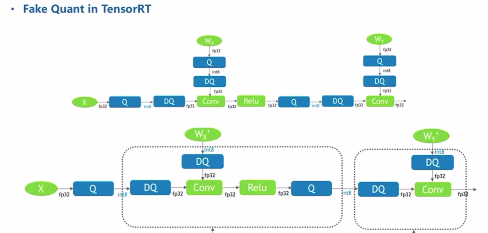
  - 通常X的Q是per tensor的，W的Q是per channel的
  - W的Q可以离线计算好
  - DQ+float conv-relu的部分可以融合为QConvRelu，输入/输出都是int8，可以放到Tensor Core去算实现加速
- FP16 & Int8
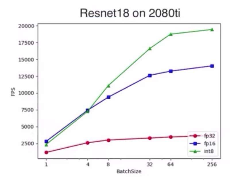
  - bs比较小的时候，还没到数据搬运瓶颈
  - bs大的时候，int8才显著

ViT

PTQ method1
- 量化矩阵乘：QK，attnV，mlp
- 计算similarity loss：皮尔逊相关系数，$sim(Y, \hat Y)$
- 计算ranking loss：监督attn的相对关系
- 交替循环采样
  - 首先计算X和W的calibration
  - fix X的calibration，采样W的calibration，得到最好的$s_w$
  - fix W的calibration，采样X的calibration，得到最好的$s_x$
  - 交替
PTQ method2
- LN
  - BN vs. LN：BN保存per-channel的statics，LN动态计算per-tensor的statics，不能融合进conv，需要独立量化
  - LN的输入数值范围分布比较大，要么损失离群点，要么拉大range损失small value的quant precision
  - 如果用per-channel量化来解，在DQ的时候恢复的数值范围不一致，还是要用浮点防止溢出
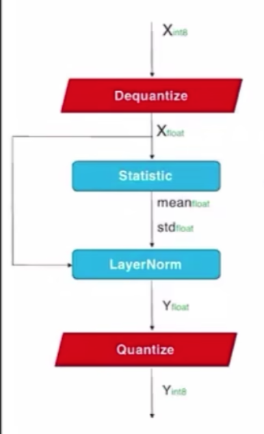
  - 把channel scale表征成2的幂数，在rescale的时候可以替换成移位操作
- Softmax
  - log2放大small value的quant range
  - i-exp将softmax转换成整数运算，因此可以直接输入前面的量化结果$softmax(s*x_q)$
  - log2量化以后的DQ可以看成
    - $x_q=-log2(x)$
    - $\hat x=2^{-x_q}$，做attnV的matmul的时候可以直接移位

pipeline

model to Qmodel：trace静态图节点

qconfig配置

build qmodel

from sparsebit.quantization import QuantModel, parse_qconfig
from model import resnet18

model = resnet18(num_classes=10)
model.load_state_dict(torch.load('pretrained.pth'))

# eval float model
# ...

# build quant model
qconfig_file = "qconfig.yaml"                 # W8A8
qconfig = parse_qconfig(qconfig_file)
qmodel = QuantModel(model, config=qconfig)

calibration：计算qparams

PTQ

# Set calibration
qmodel.prepare_calibration()
# Forward Calibrate
calibration_size = 256
cur_size = 0
if torch.cuda.is_available():
    qmodel.cuda()
for data,target in trainloader:
    if torch.cuda.is_available():
        data,target = data.cuda(),target.cuda()
    res = qmodel(data)
    cur_size += data.shape[0]
    if cur_size >= calibration_size:
        break
qmodel.calc_qparams()

QAT训练

qmodel.init_QAT()    #调用API，初始化QAT
qmodel.set_lastmodule_wbit(bit=8)    #额外规定最后一层权重的量化bit数
print(qmodel.model)    #可以在print出的模型信息中看到网络各层weight和activation的量化scale和zeropoint

# train like a float model, fake quantize等过程在QuantModel中自行完成
# Q/DQ nodes simulate quantization loss and add it to the training loss during fine-tuning

    * 得到quant model，导出onnx

    1
2
3
4
5
6
7
8
9
10
11
12
13
14
15
16
17
18
19
# Set Quantization
qmodel.set_quant(w_quant=True,a_quant=True)
correct = 0
total = 0
qmodel.eval()
with torch.no_grad():
    for data in testloader:
        image,labels = data
        if torch.cuda.is_available():
            image,labels= image.cuda(),labels.cuda()
        outputs = qmodel(image)
        _,predicted = torch.max(outputs.data,1)
        total+=labels.size(0)
        correct += (predicted == labels).sum().item()
acc1 = 100 * correct / total
print(f'Accuracy of the Quant Model on the 10000 test images: {acc1} %')

# 导出onnx
qmodel.export_onnx(torch.randn(1, 3, 224, 224), name="qresnet20.onnx")



9. homework

    * imagenet上resnet18、vgg16、mobileNetv2的PTQ掉点情况

        * Resnet18<vgg16<mobileNetv2
        * mobilenetv2量化之后掉点严重的主要原因在于该网络中的深度可分离卷积，Depthwise Conv不同输出通道的动态范围差异较大，因此采用per-tensor的量化方式将会引入较大的量化误差，从而导致精度损失严重，采用per-channel的量化能够缓解精度损失的问题。

    * 把calibration-set里面的图片换成标准高斯噪声输入, 当calibration-set大小为1, 10, 100时, 精度不是0或者很低的原因是什么呢

        * 图像预处理的Normalization操作可确保数据满足N(0,1)的高斯分布，与随机高斯噪声类似

    * moving average calibration with alpha from [0.5, 0.9, 0.99]

        * 全局的calibration MinMax好过moving average MinMax，因为step有限的情况下两者并不接近

        * alpha越大结果越差

    * int8和float16的模型latency比较

        * 二者在GPU中的速度并没有太大区别，int8的主要优势在于传输数据，相同带宽下，Int8传输的数据量是FP16的两倍
        * BatchSize较小时，其传输带宽并没有被完全利用，GPU上Int8和FP16的Throughput接近

    * QAT resnet18 with 4w4f & 2w4f

FQ-ViT: Post-Training Quantization for Fully Quantized Vision Transformer

introduction
- difficuties in quant ViT
  - serious inter-channel variation in LayerNorm inputs：一些通道的值是均值的40倍，这种fluctuation一般的量化方法解决不了，会导致large quantization error
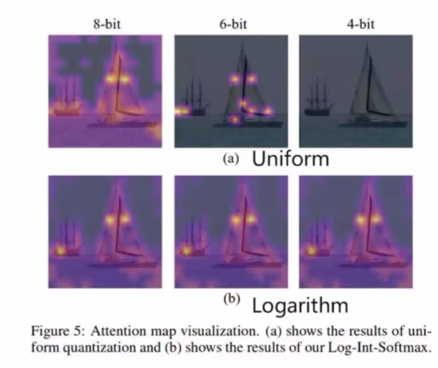
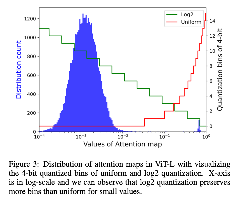
  - extreme non-uniform distribution in attention maps：attn map中大多数的units范围在0-0.01，只有少数high attention接近1，极小值在量化过程中的精度损失比较大
- propose Fully Quantized Vision Transformer (FQ-ViT)
  - PTF：power of Two Factor，能够降低LN的量化误差，计算量与layer-wise quantization一致
  - LIS：log int softmax，能够 provides higher quantization resolution for small values
  - simplify 4- bit quantization by the BitShift operator
method
- quantization preliminary
  - 量化$Q(X|b)$就是将浮点值域$X\in R$映射到量化值域$b\in q$
  - b代表bit width，那么量化值域q的分布为
    - signed：$\{-2^{b-1}, …, 2^{b-1}-1\}$
    - unsigned：$\{0,1,2,…, 2^b-1\}$
  - quantizer Q最常用的是uniform和log2
    - Uniform Quantization
      - $Q(X|b) = clip(\frac{X}{s}+zp,0,2^b-1)$
      - 两个量化参数通常是由X的分布决定，given lower bound $l$ & upper bound $u$
        
        scale $s=\frac{u-l}{2^b-1}$
        
        zero-point $zp=clip(-\frac{l}{s}, 0, 2^b-1)$
    - Log2 Quantization
      - 非线性映射
      - $Q(X|b) = sign(X)\cdot clip(-log_2\frac{|X|}{max(|X|)}, 0, 2^b-1)$
      - 会放大small value的量化区域：如果X值很大如[0.5,1]，那么对应log2的范围在[0,1]，如果X值很小如[0,0.5]那么log2的范围就在[1,inf]，可以看到log2可以放大小值的量化范围，但是对极小值有精度损失
  - this paper fully quantize ViT
    - uniform MinMax quantization is used for Conv, Linear and MatMul
    - following new proposed methods are used for LayerNorm and Softmax
- Power-of-Two Factor for LayerNorm Quantization
  - LayerNorm：$LN(x)=\frac{X-\mu_X}{\sqrt{\sigma_X^2 + \epsilon}} \cdot \gamma + \beta$
    - dynamic computing of mean & variance $\mu_X$ and $\sigma_X$
    - reaffine by trained $\gamma$ and $\beta$
    - LN层要动态norm，所以不能跟前面的线性层合并
    - look into LN的inputs：there is a serious inter-channel variation，整体的输入值分布范围很大，而且channel之间的最大值最小值差异很大
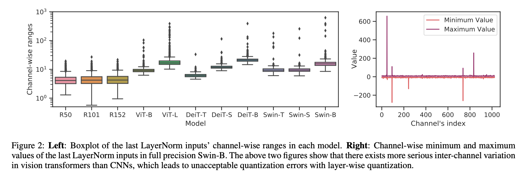
    - inter-channel的extreme variation导致layer-wise quantization有很大的quant error
      - group-wise quant和channel-wise quant：会引入更多的mean和var的计算
      - Power-of-Two Factor (PTF)：only introduce a channel-wise factor
  - $X_Q = Q(X|b) = clip(\frac{X}{2^\alpha s}+zp, 0, 2^b-1)$
    - $s=\frac{max(X)-min(X)}{2^b-1} / 2^K$
    - $zp=clip(-\frac{min(X)}{2^K s},0,2^b-1)$
    - 新引入的per-channel factor $\alpha_c= argmin ||X_c - \frac{X_c}{2^{\alpha_c} s} \cdot 2^{\alpha_c} s||_2$ among $\alpha_c\ in \ [0,1,2,…, K]$
    - hyperparam K：default K=3，可以根据需求调整，控制的是scaling factor的范围，决定了保留的精度区间，如果$X_c$的variation很大，那么对应的$\alpha_c$也要大一些
  - $X_Q$是LN的输入前量化，所以我们还可以基于它计算integer domain的LN的mean & var
    - 首先还原网络输入：$\hat X_Q = (X_Q - zp) << \alpha$
    - 网络的输入：$X = s * \hat X_Q$
    - $\mu (X) = \mu (s \hat X_Q) = \mu(\hat X_Q) s$
    - $\sigma (X) = \sigma (s \hat X_Q) = \sigma (\hat X_Q) s$
    - 这样就可以在integer domain得到LN的量化前输出：$Y=\gamma * s \frac{\hat X_Q - \mu(\hat X_Q)}{\sqrt {s^2 \sigma^2(\hat X_Q)} + \epsilon} + \beta$
  - 量化LN层
    - given quant param $s_{out}$ & $zp_{out}$
    - $Y_Q = \frac{Y}{s_{out}} + zp_{out} = \frac{\gamma s }{s_{out} \sqrt {s^2 \sigma^2(\hat X_Q)+\epsilon}} \hat X_Q + \frac{\beta\sqrt {s^2 \sigma^2(\hat X_Q)+\epsilon} - \gammas\mu(\hat X_Q)}{s_{out } * \sqrt {s^2 \sigma^2(\hat X_Q)+\epsilon}} + zp_{out} = A \hat X_Q + B + zp_{out}$
    - A近似为
      - given 目标位宽b
      - $N_1=b-1-log_2|A|$
      - $N_2= |A| 2^{N_1}$
      - $A=sign(A) \cdot \frac{N_2}{2^{N_1}}$
    - 最终的量化推理：$Y_Q=\frac{sign(A) \cdot {N_2} \hat X_Q + B*2^{N_1}}{2^{N_1}} + zp_{out}$
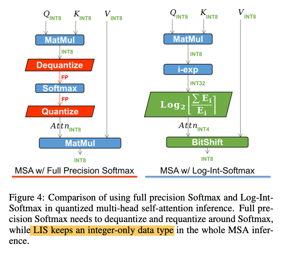
- Log-Int-Softmax for Softmax Quantization
  - look into attn map：a distribution centering at a fairly small value，然后少数离群点在1附近
  - log2 quant
    - 首先softmax自带normalization
    - 其次后面的attn*VQ这个matmul算子也可以通过bitshift来实现
  - $Attn_Q = Q(Attn|b) = clip(-log_2{Attn}, 0, 2^b-1)$
  - after quant matmul
    - $Attn V_Q = 2^{-Attn_Q} V_Q = V_Q >> Attn_Q$
    - 右移会损失精度，所以改成左移，$V_Q>>Attn_Q = V_Q << (N-Attn_Q) / 2^N$，$N=2^b-1$
  - softmax计算的优化LIS Log-Int-Softmax
    - 使用i-exp来polynomial approximation of exponential function
    - $exp(s X_Q) = s^{‘}i-exp(X_Q)$
    - Log-Int-Softmax：$LIS(s*X_Q) = N- log_2 \frac{\sum i-exp(X_Q)}{i-exp(X_Q)}$
      - integer的log2就是找bit码中第一个1，然后累加后面的值
      - i-exp就是近似表达式
        
        softmax(X)先转化：$\hat X=X-max(X)$，输入变为负数
        
        exp(X)分解：$exp(\hat X) = 2^{-z}exp(p) = exp(p)>>z$
        
        $z=\frac{-\hat X}{ln2}$
        
        $p = \hat X + zln2 \in (ln2, 0]$
        
        exp(p)近似：$L(p) = 0.3585(p+1.353)^2 + 0.344 \approx exp(p)$
        
        $exp(\hat X) \approx L(p)>>z$
        
        归一化$exp(\hat X)$得到integer softmax
      - attn的量化用了int4来节省计算量
  - 对比
    - 不量化softmax需要QK之后先dequant，移动到cpu进行浮点计算，然后再quant，再移动回GPU/NPU
    - proposed method始终在GPU里，始终是integer