families:
- [class-imbalanced CE]
- [focal loss]
- [generalized focal loss] focal loss(CE)的连续版本
- [ohem]
keras implementation:
1 | def weightedCE_loss(y_true, y_pred): |
Gradient Harmonized Single-stage Detector
动机
- one-stage detector
- 核心challenge就是imbalance issue
- imbalance between positives and negatives
- imbalance between easy and hard examples
- 这两项都能归结为对梯度的作用:a term of the gradient
- we propose a novel gradient harmonizing mechanism (GHM)
- balance the gradient flow
- easy to embed in cls/reg losses like CE/smoothL1
- GHM-C for anchor classification
- GHM-R for bounding box refinement
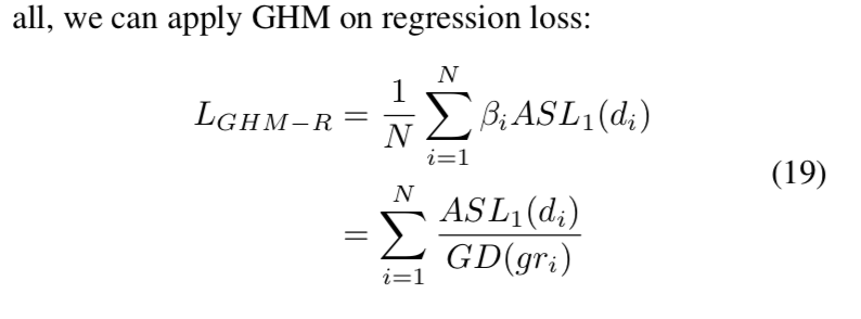
- proved substantial improvement on COCO
- 41.6 mAP
- surpass FL by 0.8
- one-stage detector
论点
imbalance issue
easy and hard:
- OHEM
- directly abandon examples
- 导致训练不充分
positive and negative
- focal loss
- 有两个超参,跟data distribution绑定
- not adaptive
通常正样本既是少量样本又是困难样本,而且可以通通归结为梯度分布不均匀的问题
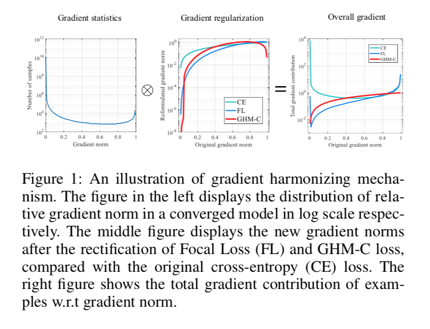
- 大量样本只贡献很小的梯度,通常对应着大量负样本,总量多了也可能会引导梯度(左图)
- hard样本要比medium样本数量大,我们通常将其看作离群点,因为模型稳定以后这些hard examples仍旧存在,他们会影响模型稳定性(左图)
- GHM的目标就是希望不同样本的gradient contribution保持harmony,相比较于CE和FL,简单样本和outlier的total contribution都被downweight,比较harmony(右图)
we propose gradient harmonizing mechanism (GHM)
- 希望不同样本的gradient contribution保持harmony
- 首先研究gradient density,按照梯度聚类样本,并相应reweight
- 针对分类和回归设计GHM-C loss和GHM-R loss
- verified on COCO
- GHM-C比CE好得多,sligtly better than FL
- GHM-R也比smoothL1好
- attains SOTA
- dynamic loss:adapt to each batch
方法
Problem Description
define gradient norm $g = |p - p^*|$
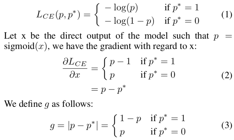
the distribution g from a converged model
- easy样本非常多,不在一个数量级,会主导global gradient
- 即使收敛模型也无法handle一些极难样本,这些样本梯度与其他样本差异较大,数量还不少,也会误导模型
Gradient Density
- define gradient density $GD(g) = \frac{1}{l_{\epsilon}(g)} \sum_{k=1} \delta_{\epsilon}(g_k,g)$
- given a gradient value g
- 统计落在中心value为$g$,带宽为$\epsilon$的范围内的梯度的样本量
- 再用带宽去norm
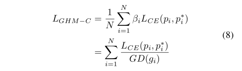
- define the gradient density harmony parameter $\beta_i = \frac{N}{GD(g_i)}$
- N是总样本量
- 其实就是与density成反比
- large density对应样本会被downweight
- define gradient density $GD(g) = \frac{1}{l_{\epsilon}(g)} \sum_{k=1} \delta_{\epsilon}(g_k,g)$
GHM-C Loss
将harmony param作为loss weight,加入现有loss
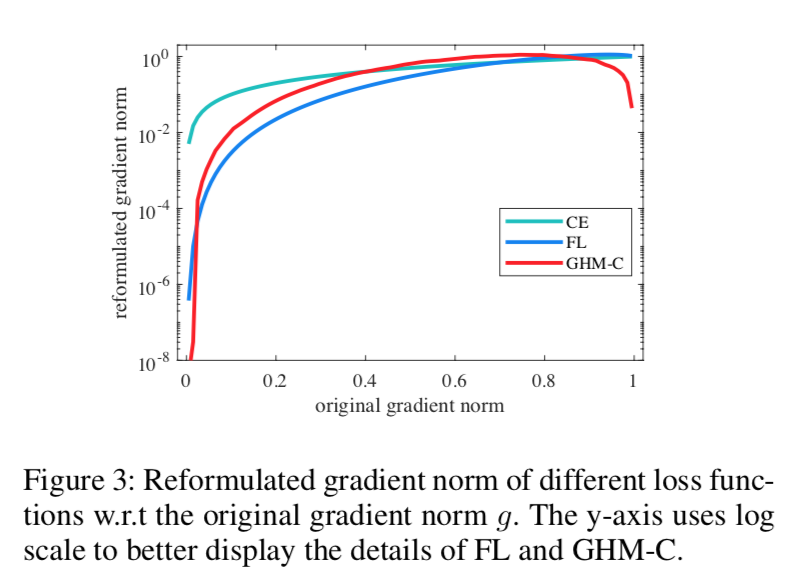
- 可以看到FL主要压简单样本(基于sample loss),GHM两头压(基于sample density)
- 最终harmonize the total gradient contribution of different density group
- dynamic wrt mini-batch:使得训练更加efficient和robust
Unit Region Approximation
- 将gradient norm [0,1]分解成M个unit region
- 每个region的宽度$\epsilon = \frac{1}{M}$
- 落在每个region内的样本数计作$R_{ind(g)}$,$ind(g)$是g所在region的start idx
- the approximate gradient density:$\hat {GD}(g) = \frac{R_{ind(g)}}{\epsilon} =R_{ind(g)}M $
approximate harmony parameter & loss:
- we can attain good performance with quite small M
- 一个密度区间内的样本可以并行计算,计算复杂度O(MN)
EMA
- 一个mini-batch可能是不稳定的
- 所以通过历史累积来更新维稳:SGDM和BN都用了EMA
- 现在每个region里面的样本使用同一组梯度,我们对每个region的样本量应用了EMA
- t-th iteraion
- j-th region
- we have $R_j^t$
- apply EMA:$S_j^t = \alpha S_j^(t-1) + (1-\alpha )R_j^t$
- $\hat GD(g) = S_{ind(g)} M$
- 这样gradient density会更smooth and insensitive to extreme data
GHM-R loss
smooth L1:
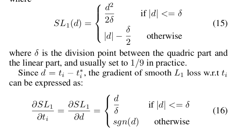
- 通常分界点设置成$\frac{1}{9}$
- SL1在线性部分的导数永远是常数,没法去distinguishing of examples
- 用$|d|$作为gradient norm则存在inf
所以先改造smooth L1:Authentic Smooth L1

- $\mu=0.02$
- 梯度范围正好在[0,1)
define gradient norm as $gr = |\frac{d}{\sqrt{d^2+\mu^2}}|$
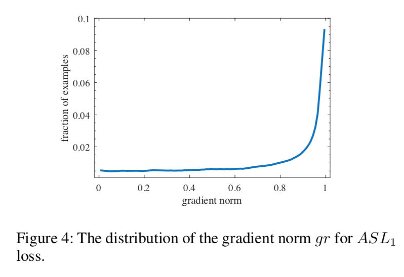
观察converged model‘s gradient norm for ASL1,发现大量是outliers
同样用gradient density进行reweighting
收敛状态下,不同类型的样本对模型的gradient contribution
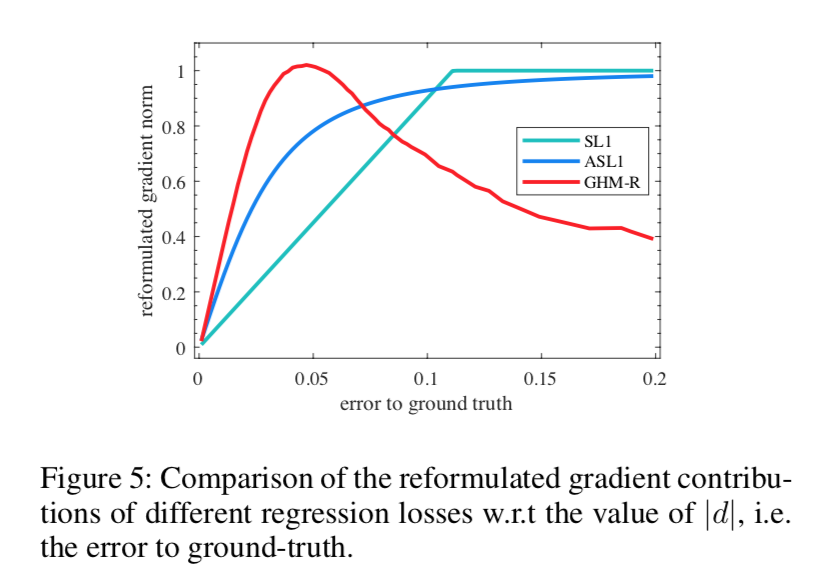
- regression是对所有正样本进行计算,主要是针对离群点进行downweighting
- 这里面的一个观点是:在regression task里面,并非所有easy样本都是不重要的,在分类task里面,easy样本大部分都是简单的背景类,但是regression分支里面的easy sample是前景box,而且still deviated from ground truth,仍旧具有充分的优化价值
- 所以GHM-R主要是upweight the important part of easy samples and downweight the outliers
实验