综述
- papers
[batch norm 2015] Batch Normalization: Accelerating Deep Network Training by Reducing Internal Covariate Shift,inceptionV2,Google Team,归一化层的始祖,加速训练&正则,BN被后辈追着打的主要痛点:approximation by mini-batch,test phase frozen
[layer norm 2016] Layer Normalization,Toronto+Google,针对BN不适用small batch和RNN的问题,主要用于RNN,在CNN上不好,在test的时候也是active的,因为mean&variance由于当前数据决定,有负责rescale和reshift的layer params
[weight norm 2016] Weight normalization: A simple reparameterization to accelerate training of deep neural networks,OpenAI,
[cosine norm 2017] Cosine Normalization: Using Cosine Similarity Instead of Dot Product in Neural Networks,中科院,
[instance norm 2017] Instance Normalization: The Missing Ingredient for Fast Stylization,高校report,针对风格迁移,IN在test的时候也是active的,而不是freeze的,单纯的instance-independent norm,没有layer params
[group norm 2018] Group Normalization,FAIR Kaiming,针对BN在small batch上性能下降的问题,提出batch-independent的
[weight standardization 2019] Weight Standardization,Johns Hopkins,
[batch-channel normalization & weight standardization 2020] BCN&WS: Micro-Batch Training with Batch-Channel Normalization and Weight Standardization,Johns Hopkins,
why Normalization
独立同分布:independent and identically distribute
白化:whitening([PCA whitening][http://ufldl.stanford.edu/tutorial/unsupervised/PCAWhitening/])
- 去除特征之间的相关性
- 使所有特征具有相同的均值和方差
样本分布变化:Internal Covariate Shift
- 对于神经网络的各层输入,由于stacking internel byproduct,每层的分布显然各不相同,但是对于某个特定的样本输入,他们所指示的label是不变的
即源空间和目标空间的条件概率是一致的,但是边缘概率是不同的
每个神经元的数据不再是独立同分布,网络需要不断适应新的分布,上层神经元容易饱和:网络训练又慢又不稳定
how to Normalization
preparation
- unit:一个神经元(一个op),输入[b,N,C_in],输出[b,N,1]
- layer:一层的神经元(一系列op,$W\in R^{M*N}$),在channel-dim上concat当前层所有unit的输出[b,N,C_out]
- dims
- b:batch dimension
- N:spatial dimension,1/2/3-dims
- C:channel dimension
- unified representation:本质上都是对数据在规范化
- $h = f(g*\frac{x-\mu}{\sigma}+b)$:先归一化,在rescale & reshift
- $\mu$ & $\sigma$:compute from上一层的特征值
- $g$ & $b$:learnable params基于当前层
- $f$:neurons’ weighting operation
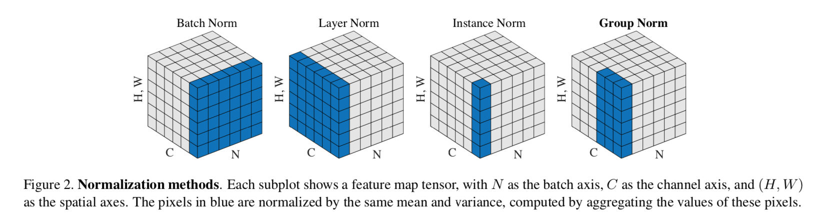
- 各方法的主要区别在于mean & variance的计算维度
对数据
- BN:以一层每个神经元的输出为单位,即每个channel的mean&var相互独立
- LN:以一层所有神经元的输出为单位,即每个sample的mean&var相互独立
- IN:以每个sample在每个神经元的输出为单位,每个sample在每个channel的mean&var都相互独立
- GN:以每个sample在一组神经元的输出为单位,一组包含一个神经元的时候变成IN,一组包含一层所有神经元的时候就是LN
示意图:
对权重
- WN:将权重分解为单位向量和一个固定标量,相当于神经元的任意输入vec点乘了一个单位vec(downscale),再rescale,进一步地相当于没有做shift和reshift的数据normalization
- WS:对权重做全套(归一化再recale),比WN多了shift,“zero-center is the key”
对op
CosN:
将线性变换op替换成cos op:$f_w(x) = cos
数学本质上又退化成了只有downscale的变换,表征能力不足
Whitening白化
purpose
- images的adjacent pixel values are highly correlated,thus redundant
- linearly move the origin distribution,making the inputs share the same mean & variance
method
首先进行PCA预处理,去掉correlation
mean on sample(注意不是mean on image)
协方差矩阵
奇异值分解svd(S)
- $\Sigma$为对角矩阵,对角上的元素为奇异值
- $U=[u_1,u_2,…u_N]$中是奇异值对应的正交向量
投影变换
- 取投影矩阵$U_p$ from $U$,$U_p \in R^{N*d}$表示将数据空间从N维投影到$U_p$所在的d维空间上
recover(投影逆变换)
        * 取投影矩阵$U_r=U_p^T$,就是将 数据空间从d维空间再投影回N维空间上

* PCA白化:

    * 对PCA投影后的新坐标,做归一化处理:基于特征值进行缩放
        $$
        X_{PCAwhite} = \Sigma^{-\frac{1}{2}}X^{'} =  \Sigma^{-\frac{1}{2}}U^TX
        $$

    * $X_{PCAwhite}$的协方差矩阵$S_{PCAwhite} = I$,因此是去了correlation的

* ZCA白化:在上一步做完之后,再把它变换到原始空间,所以ZCA白化后的特征图更接近原始数据

    * 对PCA白化后的数据,再做一步recover
        $$
        X_{ZCAwhite} = U X_{PCAwhite}
        $$

    * 协方差矩阵仍旧是I,合法白化
Layer Normalization
动机
BN reduces training time
- compute by each neuron
- require moving average
- depend on mini-batch size
- how to apply to recurrent neural nets
propose layer norm
- [unlike BN] compute by each layer
- [like BN] with adaptive bias & gain
- [unlike BN] perform the same computation at training & test time
- [unlike BN] straightforward to apply to recurrent nets
- work well for RNNs
论点
- BN
- reduce training time & serves as regularizer
- require moving average:introduce dependencies between training cases
- the approxmation of mean & variance expectations constraints on the size of a mini-batch
- intuition
- norm layer提升训练速度的核心是限制神经元输入输出的变化幅度,稳定梯度
- 只要控制数据分布,就能保持训练速度
- BN
方法
- compute over all hidden units in the same layer
- different training cases have different normalization terms
- 没啥好说的,就是在channel维度计算norm
- further的GN把channel维度分组做norm,IN在直接每个特征计算norm
- gain & bias
- 也是在对应维度:(hwd)c-dim
- https://tobiaslee.top/2019/11/21/understanding-layernorm/
- 后续有实验发现,去掉两个learnable rescale params反而提点
- 考虑是在training set上的过拟合
实验
- RNN上有用
- CNN上比没有norm layer好,但是没有BN好:因为channel是特征维度,特征维度之间有明显的有用/没用,不能简单的norm
Weight Normalization: A Simple Reparameterization to Accelerate Training of Deep Neural Networks
- 动机
- reparameterizing the weights
- decouple length & direction
- no dependency between samples which suits well for
- recurrent
- reinforcement
- generative
- no additional memory and computation
- testified on
- MLP with CIFAR
- generative model VAE & DRAW
- reinforcement DQN
- reparameterizing the weights
- 论点
- a neuron:
- get inputs from former layers(neurons)
- weighted sum over the inputs
- add a bias
- elementwise nonlinear transformation
- batch outputs:one value per sample
- intuition of normalization:
- give gradients that are more like whitened natural gradients
- BN:make the outputs of each neuron服从std norm
- our WN:
- inspired by BN
- does not share BN’s across-sample property
- no addition memory and tiny addition computation
- a neuron:
Instance Normalization: The Missing Ingredient for Fast Stylization
动机
- stylization:针对风格迁移网络
- with a small change:swapping BN with IN
- achieve qualitative improvement
论点
- stylized image
- a content image + a style image
- both style and content statistics are obtained from a pretrained CNN for image classification
- methods
- optimization-based:iterative thus computationally inefficient
- generator-based:single pass but never as good as
- our work
- revisit the feed-forward method
- replace BN in the generator with IN
- keep them at test time as opposed to freeze
- stylized image
方法
formulation
- given a fixed stype image $x_0$
- given a set of content images $x_t, t= 1,2,…,n$
- given a pre-trained CNN
- with a variable z controlling the generation of stylization results
- compute the stylied image g($x_t$, z)
- compare the statistics:$min_g \frac{1}{n} \sum^n_{t=1} L(x_0, x_t, g(x_t, z))$
- comparing target:the contrast of the stylized image is similar to the constrast of the style image
observations
- the more training examples, the poorer the qualitive results
- the result of stylization still depent on the constrast of the content image
intuition
- 风格迁移本质上就是将style image的contrast用在content image的:也就是rescale content image的contrast
constrast是per sample的:$\frac{pixel}{\sum pixels\ on\ the\ map}$
BN在norm的时候将batch samples搅合在了一起
IN
- instance-specfic normalization
also known as contrast normalization
就是per image做标准化,没有trainable/frozen params,在test phase也一样用
Group Normalization
动机
- for small batch size
- do normalization in channel groups
- batch-independent
- behaves stably over different batch sizes
approach BN’s accuracy

论点
- BN
- requires sufficiently large batch size (e.g. 32)
- Mask R-CNN frameworks use a batch size of 1 or 2 images because of higher resolution, where BN is “frozen” by transforming to a linear layer
- synchronized BN 、BR
- LN & IN
- effective for training sequential models or generative models
- but have limited success in visual recognition
- GN能转换成LN/IN
- WN
- normalize the filter weights, instead of operating on features
- BN
方法
group
- it is not necessary to think of deep neural network features as unstructured vectors
- 第一层卷积核通常存在一组对称的filter,这样就能捕获到相似特征
- 这些特征对应的channel can be normalized together
- it is not necessary to think of deep neural network features as unstructured vectors
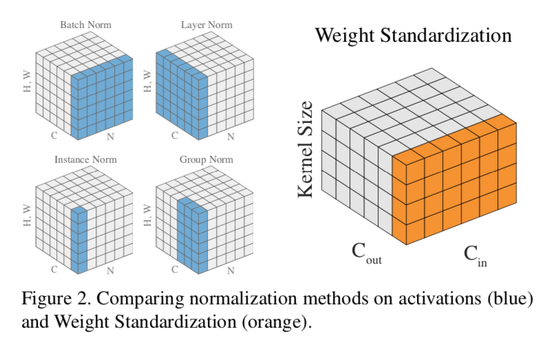
normalization
transform the feature x:$\hat x_i = \frac{1}{\sigma}(x_i-\mu_i)$
the mean and the standard deviation:
the set $S_i$
- BN:
- $S_i=\{k|k_C = i_C\}$
- pixels sharing the same channel index are normalized together
- for each channel, BN computes μ and σ along the (N, H, W) axes
- LN
- $S_i=\{k|k_N = i_N\}$
- pixels sharing the same batch index (per sample) are normalized together
- LN computes μ and σ along the (C,H,W) axes for each sample
- IN
- $S_i=\{k|k_N = i_N, k_C=i_C\}$
- pixels sharing the same batch index and the same channel index are normalized together
- LN computes μ and σ along the (H,W) axes for each sample
- GN
- $S_i=\{k|k_N = i_N, [\frac{k_C}{C/G}]=[\frac{i_C}{C/G}]\}$
- computes μ and σ along the (H, W ) axes and along a group of C/G channels
- BN:
linear transform
- to keep representational ability
- per channel
- scale and shift:$y_i = \gamma \hat x_i + \beta$

relation
- to LN
- LN assumes all channels in a layer make “similar contributions”
- which is less valid with the presence of convolutions
- GN improved representational power over LN
- to IN
- IN can only rely on the spatial dimension for computing the mean and variance
- it misses the opportunity of exploiting the channel dependence
- 【QUESTION】BN也没考虑通道间的联系啊,但是计算mean和variance时跨了sample
- to LN
implementation
- reshape
- learnable $\gamma \& \beta$
- computable mean & var

实验
- GN相比于BN,training error更低,但是val error略高于BN
- GN is effective for easing optimization
- loses some regularization ability
- it is possible that GN combined with a suitable regularizer will improve results
- 选取不同的group数,所有的group>1均好于group=1(LN)
- 选取不同的channel数(C/G),所有的channel>1均好于channel=1(IN)
- Object Detection
- frozen:因为higher resolution,batch size通常设置为2/GPU,这时的BN frozen成一个线性层$y=\gamma(x-\mu)/\sigma+beta$,其中的$\mu$和$sigma$是load了pre-trained model中保存的值,并且frozen掉,不再更新
- denote as BN*
- replace BN* with GN during fine-tuning
- use a weight decay of 0 for the γ and β parameters
- GN相比于BN,training error更低,但是val error略高于BN
WS: Weight Standardization
动机
- accelerate training
- micro-batch:
- 以BN with large-batch为基准
- 目前BN with micro-batch及其他normalization methods都不能match这个baseline
- operates on weights instead of activations
- 效果
- match or outperform BN
- smooth the loss
论点
two facts
- BN的performance gain与reduction of internal covariate shift没什么关系
- BN使得optimization landscape significantly smoother
- 因此our target is to find another technique
- achieves smooth landscape
- work with micro-batch
normalization methods
- focus on activations
- 不展开
focus on weights
- WN:just length-direction decoupling
- focus on activations
方法
Lipschitz constants
- BN reduces the Lipschitz constants of the loss function
- makes the gradient more Lipschitz
- BN considers the Lipschitz constants with respect to activations,not the weights that the optimizer is directly optimizing
our inspiration
- standardize the weights也同样能够smooth the landscape
- 更直接
- smoothing effects on activations and weights是可以累积的,因为是线性运算
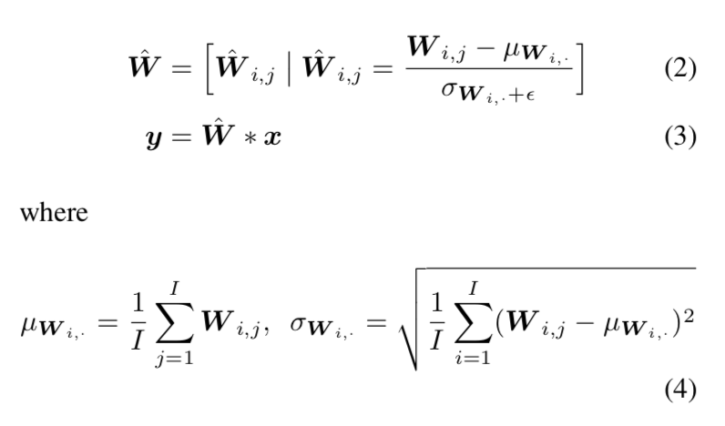
Weight Standardization
- reparameterize the original weights $W$
- 对卷积层的权重参数做变换,no bias
- $W \in R^{O * I}$
- $O=C_{out}$
- $I=C_{in}*kernel_size$
- optimize the loss on $\hat W$
- compute mean & var on I-dim
只做标准化,无需affine,因为默认后续还要接一个normalization layer对神经元进行refine
- reparameterize the original weights $W$
WS normalizes gradients
拆解:
- eq5:$W$ to $\dot W$,减均值,zero-centered
- eq6:$\dot W$ to $\hat W$,除方差,one-varianced
- eq8:$\delta \hat W$由前一步的梯度normalize得到
- eq9:$\delta \dot W$也由前一步的梯度normalize
最终用于梯度更新的梯度是zero-centered
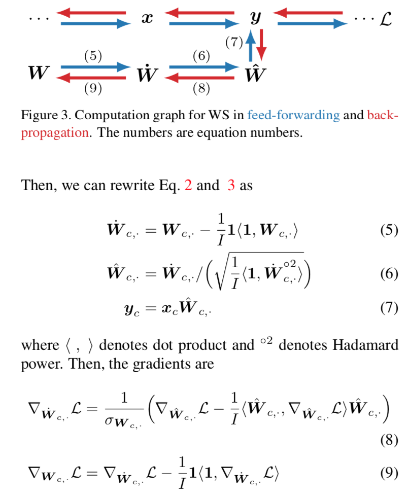
WS smooths landscape
- 判定是否smooth就看Lipschitz constant的大小
- eq5和eq6都能reduce the Lipschitz constant
- 其中eq5 makes the major improvements
- eq6 slightly improves,因为计算量不大,所以保留
实验
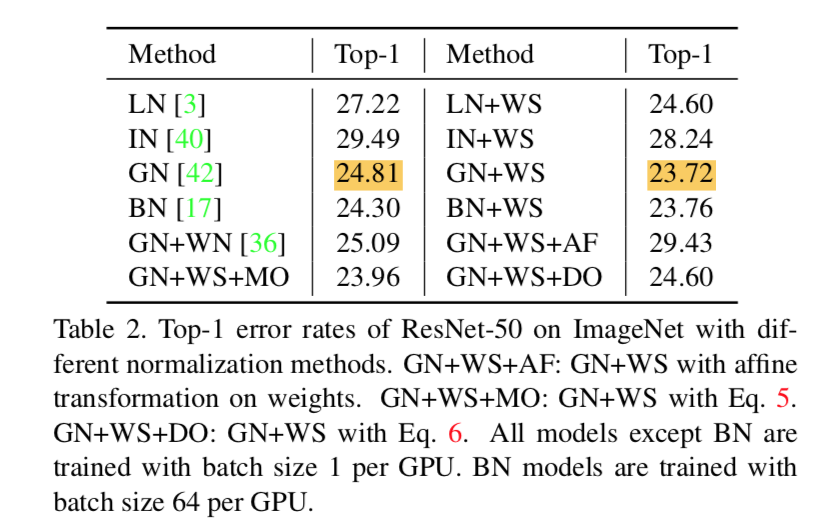
ImageNet
- BN的batchsize是64,其余都是1,其余的梯度更新iterations改成64——使得参数更新次数同步
- 所有的normalization methods加上WS都有提升
- 裸的normalization methods里面batchsize1的GN最好,所以选用GN+WS做进一步实验
GN+WS+AF:加上conv weight的affine会harm
code
1 | # official release |