综述
papers
[V1] Going Deeper with Convolutions, 6.67% test error
[V2] Batch Normalization: Accelerating Deep Network Training by Reducing Internal Covariate Shift, 4.8% test error
[V3] Rethinking the Inception Architecture for Computer Vision, 3.5% test error
[V4] Inception-v4, Inception-ResNet and the Impact of Residual Connections on Learning, 3.08% test error
[Xception] Xception: Deep Learning with Depthwise Separable Convolutions
[EfficientNet] EfficientNet: Rethinking Model Scaling for Convolutional Neural Networks
[EfficientDet] EfficientDet: Scalable and Efficient Object Detection
[EfficientNetV2] EfficientNetV2: Smaller Models and Faster Training
大体思路
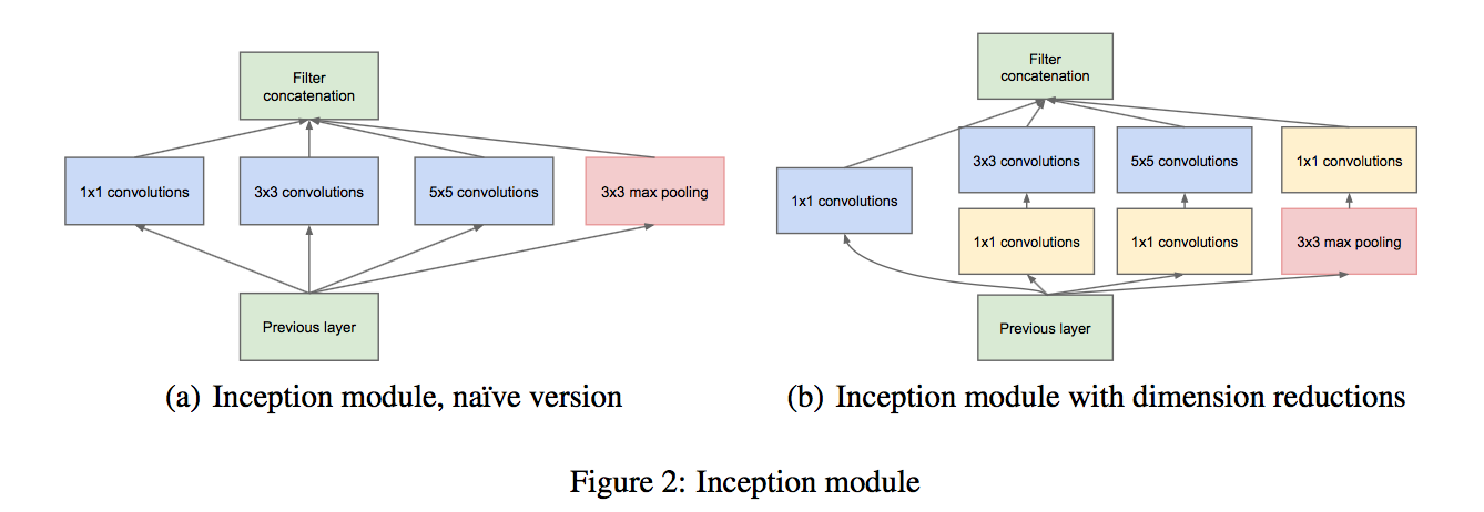
- inception V1:打破传统的conv block,设计了Inception block,将1*1、3*3、5*5的卷积结果concat,增加网络宽度
- inception V2:加入了BN层,减少Internal Covariate Shift,用两个3*3替代5*5,降低参数量
- inception V3:提出分解Factorization,7*7改成7*1和1*7,参数减少加速计算,增加网络深度和非线性
- inception V4:结合Residual Connection
- Xception:针对inception V3的分解结构的改进,使用可分离卷积
- EfficientNet:主要研究model scaling,针对网络深度、宽度、图像分辨率,有效地扩展CNN
- EfficientDet:将EfficientNet从分类任务扩展到目标检测任务
review
review0122:conv-BN层合并运算
reference:https://nenadmarkus.com/p/fusing-batchnorm-and-conv/
freezed BN可以看成1x1的卷积运算
两个线性运算是可以合并的
given $W_{conv} \in R^{CC_{prev}kk}$,$b_{conv} \in R^C $,$W_{bn}\in R^{CC}$,$b_{bn}\in R^C$
V1: Going deeper with convolutions
动机
- improved utilization of the computing resources
- increasing the depth and width of the network while keeping the computational budget
论点
- the recent trend has been to increase the number of layers and layer size, while using dropout to address the problem of overfitting
- major bottleneck:large network,large number of params,limited dataset,overfitting
- methods use filters of different sizes in order to handle multiple scales
- NiN use 1x1 convolutional layers to easily integrate in the current CNN pipelines
- we use 1x1 convs with a dual purpose of dimension reduction
方法
Architectural
- 1x1 conv+ReLU for compute reductions
an alternative parallel pooling path since pooling operations have been essential for the success
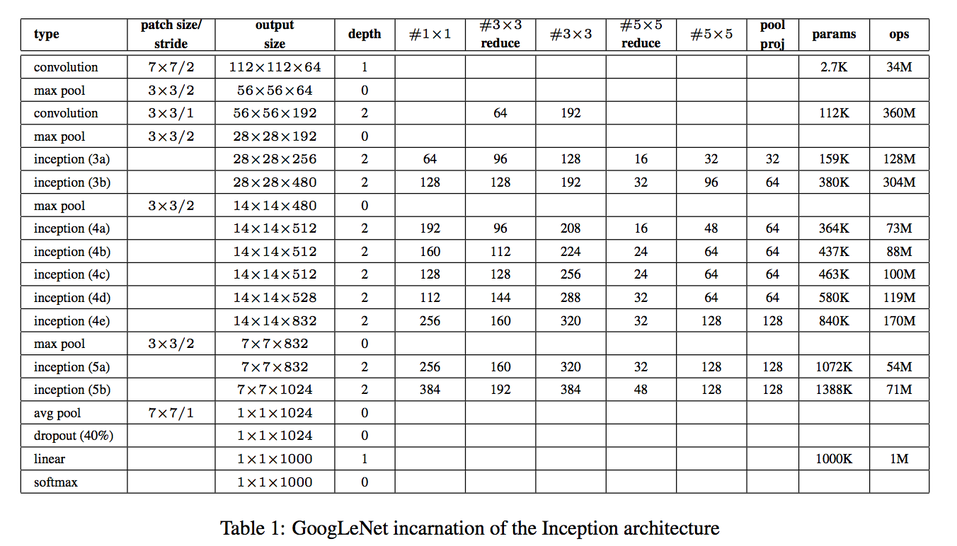
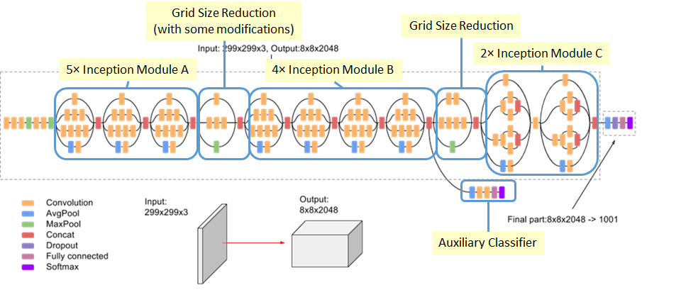
overall architecture :
细节:
rectified linear activation
mean subtraction
a move from fully connected layers to average pooling improves acc
the use of dropout remained essential
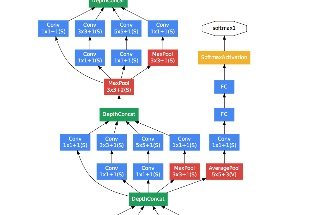
adding auxiliary classifiers(on 4c&4d) with a discount weight
- 5x5 avg pool, stride 3
- 1x1 conv+relu, 128 filters
- 1024 fc+relu
- 70% dropout
1000 fc+softmax
asynchronous stochastic gradient descent with 0.9 momentum
fixed learning rate schedule (de- creasing the learning rate by 4% every 8 epochs
photometric distortions useful to combat overfitting
random interpolation methods for resizing
V2: Batch Normalization: Accelerating Deep Network Training by Reducing Internal Covariate Shift
动机
- use much higher learning rates
- be less careful about initialization
- also acts as a regularizer, eliminating the need for Dropout
论点
SGD:optimizes the parameters $\theta$ of the network, so as to minimize the loss
梯度更新:,$x_i$ is the full set
batch approximation:use $\frac{1}{m} \sum_M \frac{\partial loss(\theta)}{\partial \theta}$,$x_i$ is the mini-batch set
- quality improves as the batch size increases
- computation over a batch is much more efficient than m computations for individual examples
- the learning rate and the initial values require careful tuning
Internal covariate shift
- the input distribution of the layers changes
- consider a gradient descent step above,$x$的数据分布改变了,$\theta$就要相应地 readjust to compensate for the change in the distribution of x
activation
- 对于神经元$z = sigmoid(Wx+b)$,前面层的参数变化,很容易导致当前神经元的响应值不在有效活动区间,从而导致过了当前激活函数以后梯度消失,slow down the convergence
- In practice, using ReLU & careful initialization & small learning rates
- 如果我们能使得the distribution of nonlinearity inputs remains more stable as the network trains,就不会出现神经元饱和的问题
whitening
- 对training set的预处理:linearly transformed to have zero means and unit variances, and decorrelated
- 使得输入数据的分布保持稳定,normal distribution
- 同时去除了数据间的相关性
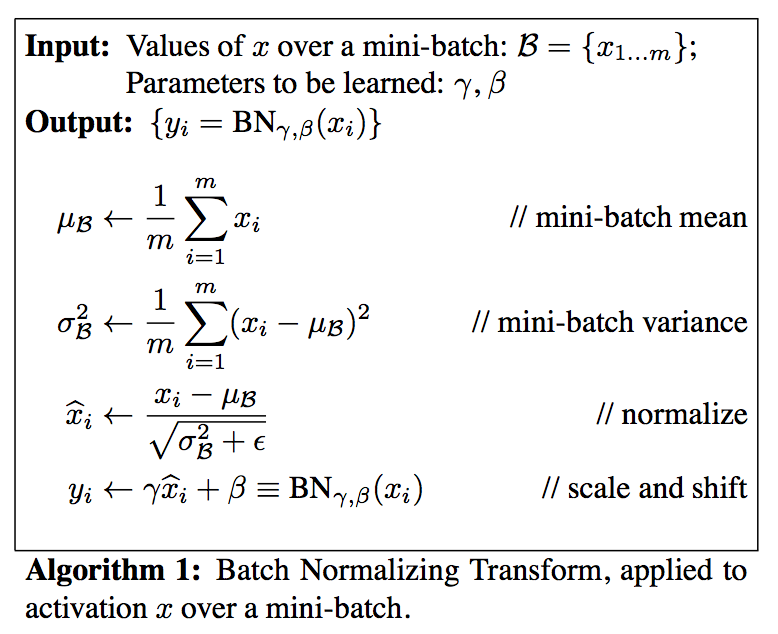
batch normalization
- fixes the means and variances of layer inputs
- reducing the dependence of gradients on the scale of the parameters or of their initial values
- makes it possible to use saturating nonlinearities
* full whitening of each layer is costly
* so we normalize each layer independently, full set--> mini-batch
* standard normal distribution并不是每个神经元所需的(如identity transform):introduce, for each activation $x(k)$ , a pair of parameters $\gamma(k)$, $\beta(k)$, which scale and shift the normalized value to maintain the representation ability of the neuron
* for convolutional networks
* we add the BN transform immediately before the nonlinearity, $z = g(Wx+b)$ to $z = g(BN(Wx))$
* since we normalize $Wx+b$, the bias b can be ignored
* obey the convolutional property——different elements of the same feature map, at different locations, are normalized in the same way
* We learn a pair of parameters $\gamma(k)$ and $\beta(k)$ **per feature map**, rather than per activation
* properties
* back-propagation through a layer is unaffected by the scale of its parameters
* Moreover, larger weights lead to smaller gradients, thus stabilizing the parameter growth
* regularizes the model:因为网络中mini-batch的数据之间是有互相影响的而非independent的
方法
batch normalization
- full whitening of each layer is costly
- so we normalize each layer independently, full set—> mini-batch
standard normal distribution并不是每个神经元所需的(如identity transform):introduce, for each activation $x(k)$ , a pair of parameters $\gamma(k)$, $\beta(k)$, which scale and shift the normalized value to maintain the representation ability of the neuron
bp:
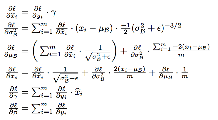
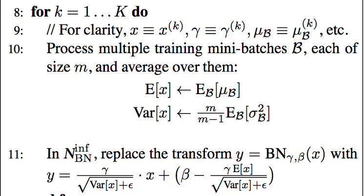
inference阶段:
- 首先两个可学习参数$\gamma$和$\beta$是定下来的
而均值和方差不再通过输入数据来计算,而是载入训练过程中维护的参数(moving averages)
for convolutional networks
we add the BN transform immediately before the nonlinearity, $z = g(Wx+b)$ to $z = g(BN(Wx))$
since we normalize $Wx+b$, the bias b can be ignored
- obey the convolutional property——different elements of the same feature map, at different locations, are normalized in the same way
- We learn a pair of parameters $\gamma(k)$ and $\beta(k)$ per feature map, rather than per activation
properties
- back-propagation through a layer is unaffected by the scale of its parameters
- Moreover, larger weights lead to smaller gradients, thus stabilizing the parameter growth
- regularizes the model:因为网络中mini-batch的数据之间是有互相影响的而非independent的
V3: Rethinking the Inception Architecture for Computer Vision
动机
- go deeper and wider:
- enough labeled data
- computational efficiency
- parameter count
- to scale up networks
- utilizing the added computation as efficiently
- give general design principles and optimization ideas
- factorized convolutions
- aggressive regularization
- go deeper and wider:
论点
- GoogleNet does not provide a clear description about the contributing factors that lead to the various design
方法
General Design Principles
- Avoid representational bottlenecks:特征图尺寸应该gently decrease,resolution的下降必须伴随着channel数的上升,避免使用max pooling层进行下采样,因为这样导致信息损失较大
- Higher dimensional representations are easier to process locally within a network. Increasing the activa- tions per tile in a convolutional network allows for more disentangled features. The resulting networks will train faster:前半句懂了,high-reso的特征图focus在局部信息,后半句不懂,根据上一篇paper,用了batch norm以后,scale up神经元不影响bp,同时会lead to smaller gradients,为啥能加速?
- Spatial aggregation can be done over lower dimensional embeddings:adjacent unit之间有strong correlation,所以可以reduce the dimension of the input representation before the spatial aggregation,不会有太大的信息损失,并且promotes faster learning
- The computational budget should therefore be distributed in a balanced way between the depth and width of the network.
Factorizing Convolutions Filter Size
- into smaller convolutions
- 大filter都可以拆解成多个3x3
- 单纯去等价线性分解可以不使用非线性activation,但是我们使用了batch norm(increase variaty),所以观察到使用ReLU以后拟合效果更好
- into Asymmetric Convolutions
- n*n的filter拆解成1*n和n*1
- this factorization does not work well on early layers, but gives very good results on medium grid-sizes (ranges between 12 and 20, using 1x7 and 7x1
- into smaller convolutions
Utility of Auxiliary Classifiers
- did not result in improved convergence early in the training:训练开始阶段没啥用,快收敛时候有点点acc提升
- removal of the lower auxiliary branch did not have any adverse effect on the final quality:拿掉对最终结果没影响
- 所以最初的设想(help evolving the low-level features) 是错的,仅仅act as regularizer,auxiliary head里面加上batch norm会使得最终结果better
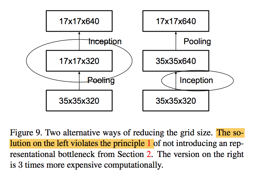
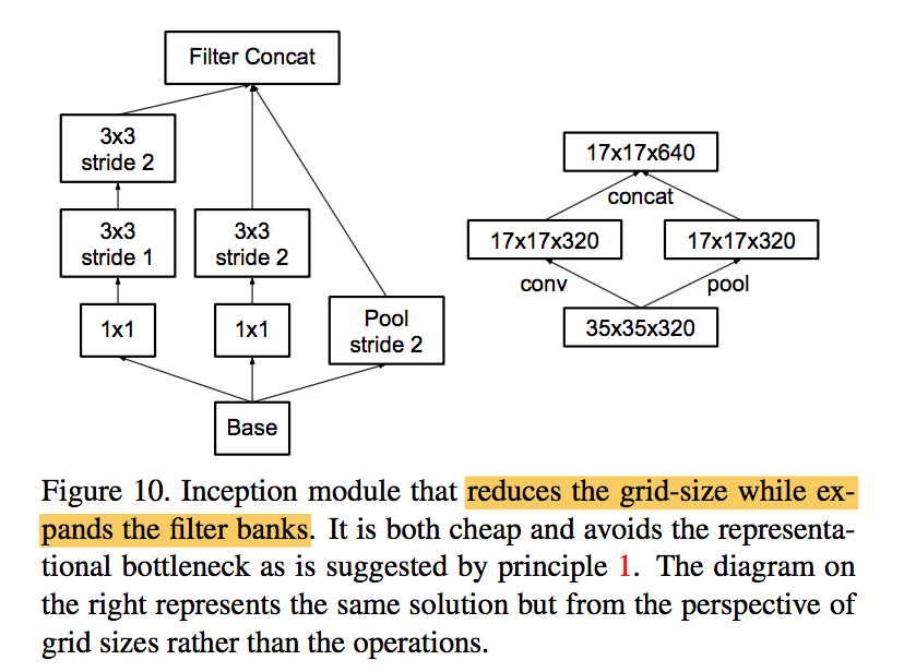
Efficient Grid Size Reduction下采样模块不再使用maxpooling
dxdxk feature map expand to (d/2)x(d/2)x2k:
- 1x1x2k conv,stride2 pool:kxdxdx2k computation
- 1x1x2k stride2 conv:kx(d/2)x(d/2)x2k computation,计算量下降,但是违反principle1
- parallel stride P and C blocks:kx(d/2)x(d/2)xk computation,符合principle1:reduces the grid-size while expands the filter banks
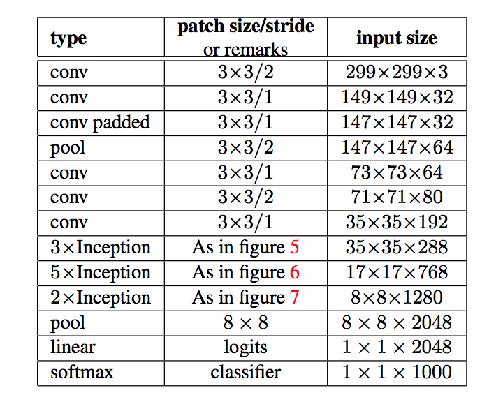
Inception-v3
- 开头的7x7conv已经换成了多个3x3
- 中间层featuremap降维到17x17的时候,开始用Asymmetric Factorization block
- 到8x8的时候,做了expanding the filter bank outputs
Label Smoothing (https://zhuanlan.zhihu.com/p/116466239)
used the uniform distribution $u(k)=1/K$
对于softmax公式:$p(k)=\frac{exp(y_k)}{\sum exp(y_i)}$,这个loss训练的结果就是$y_k$无限趋近于1,其他$y_i$无限趋近于0,
交叉熵loss:$ce=\sum -y_{gt}log(y_k)$,加了label smoothing以后,loss上增加了阴性样本的regularization,正负样本的最优解被限定在有限值,通过抑制正负样本输出差值,使得网络有更强的泛化能力。
V4: Inception-v4, Inception-ResNet and the Impact of Residual Connections on Learning
动机
- residual:whether there are any benefit in combining the Inception architecture with residual connections
- inceptionV4:simplify the inception blocks
论点
- residual connections seems to improve the training speed greatly:但是没有也能训练深层网络
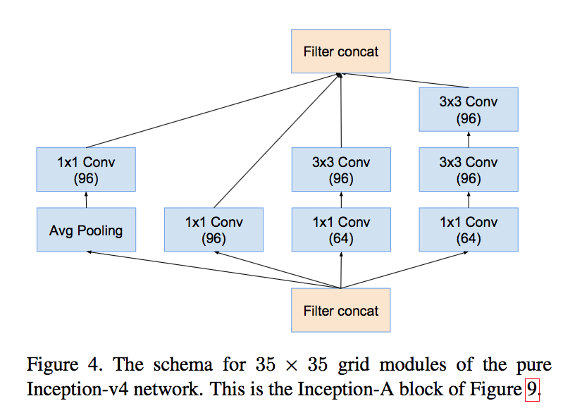
- made uniform choices for the Inception blocks for each grid size
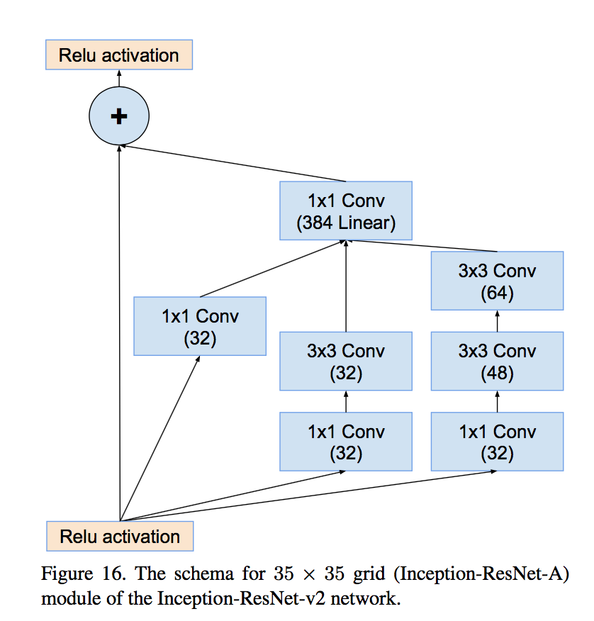
- Inception-A for 35x35
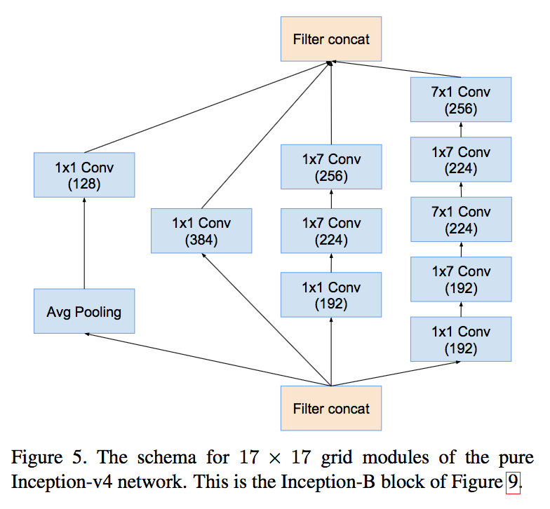
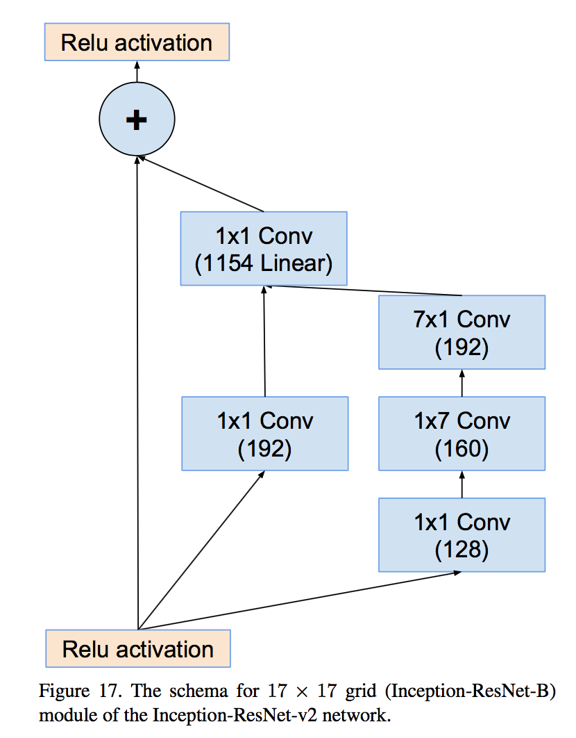
- Inception-B for 17x17
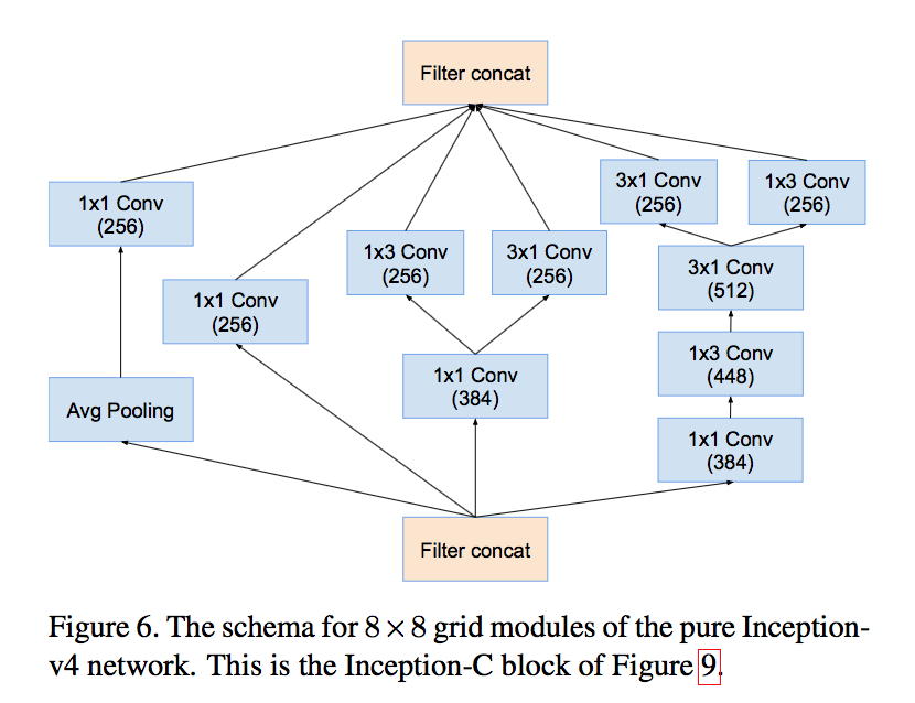
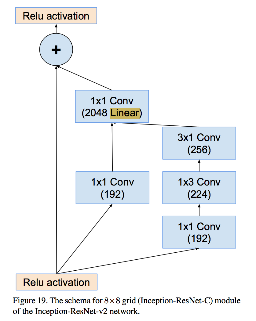
- Inception-C for 8x8
- for residual versions
- use cheaper Inception blocks for residual versions:简化module,因为identity部分(直接相连的线)本身包含丰富的特征信息
- 没有使用pooling
- replace the filter concatenation stage of the Inception architecture with residual connections:原来block里面的concatenation主体放在残差path中
- Each Inception block is followed by filter-expansion layer (1 × 1 convolution without activation) to match the depth of the input for addition:相加之前保证channel数一致
- used batch-normalization only on top of the traditional layers, but not on top of the summations:浪费内存
- number of filters exceeded 1000 causes instabilities
- scaling down the residuals before adding by factors between 0.1 and 0.3:残差通道响应值不要太大
blocks
V4 ABC:
Res ABC:
Xception: Deep Learning with Depthwise Separable Convolutions
动机
- Inception modules have been replaced with depthwise separable convolutions
- significantly outperforms Inception V3 on a larger dataset
- due to more efficient use of model parameters
论点
early LeNet-style models
- simple stacks of convolutions for feature extraction and max-pooling operations for spatial sub-sampling
- increasingly deeper
complex blocks
- Inception modules inspired by NiN
- be capable of learning richer repre- sentations with less parameters
The Inception hypothesis
- a single convolution kernel is tasked with simultaneously mapping cross-channel correlations and spatial correlations
- while Inception factors it into a series of operations that independently look at cross-channel correlations(1x1 convs) and at spatial correlations(3x3/5x5 convs)
suggesting that cross-channel correlations and spatial correlations are sufficiently decoupled that it is preferable not to map them jointly
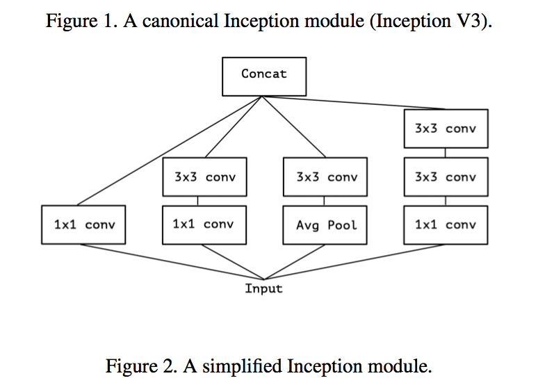
inception block先用1x1的conv将原输出映射到3-4个lower space(cross-channel correlations),然后在这些小的3d spaces上做regular conv(maps all correlations )——进一步假设,彻底解耦,第二步只做spatial correlations
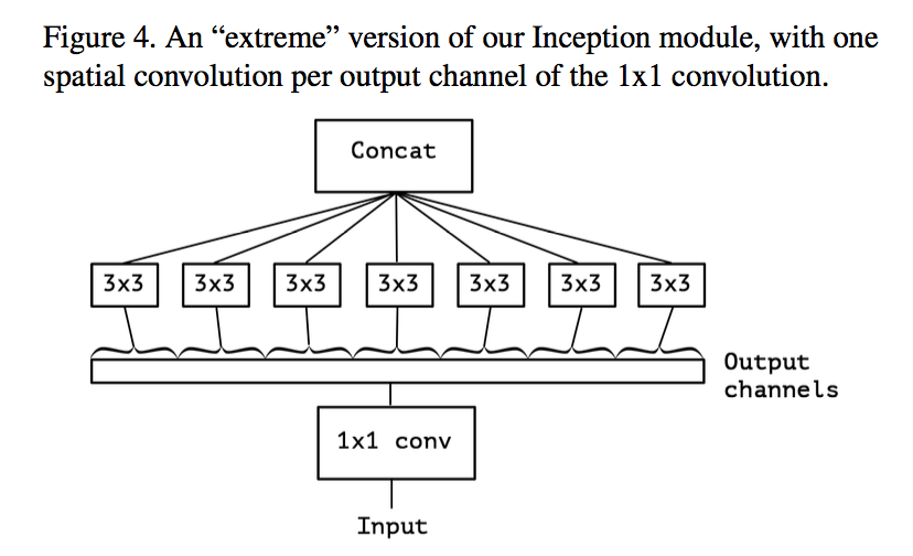
main differences between “extreme ” Inception and depthwise separable convolution
- order of the operations:1x1 first or latter
- non-linearity:depthwise separable convolutions are usually implemented without non-linearities【QUESTION:这和MobileNet里面说的不一样啊,M里面的depthwise也是每层都带了BN和ReLU的】
要素
- Convolutional neural networks
- The Inception family
- Depthwise separable convolutions
- Residual connections
方法
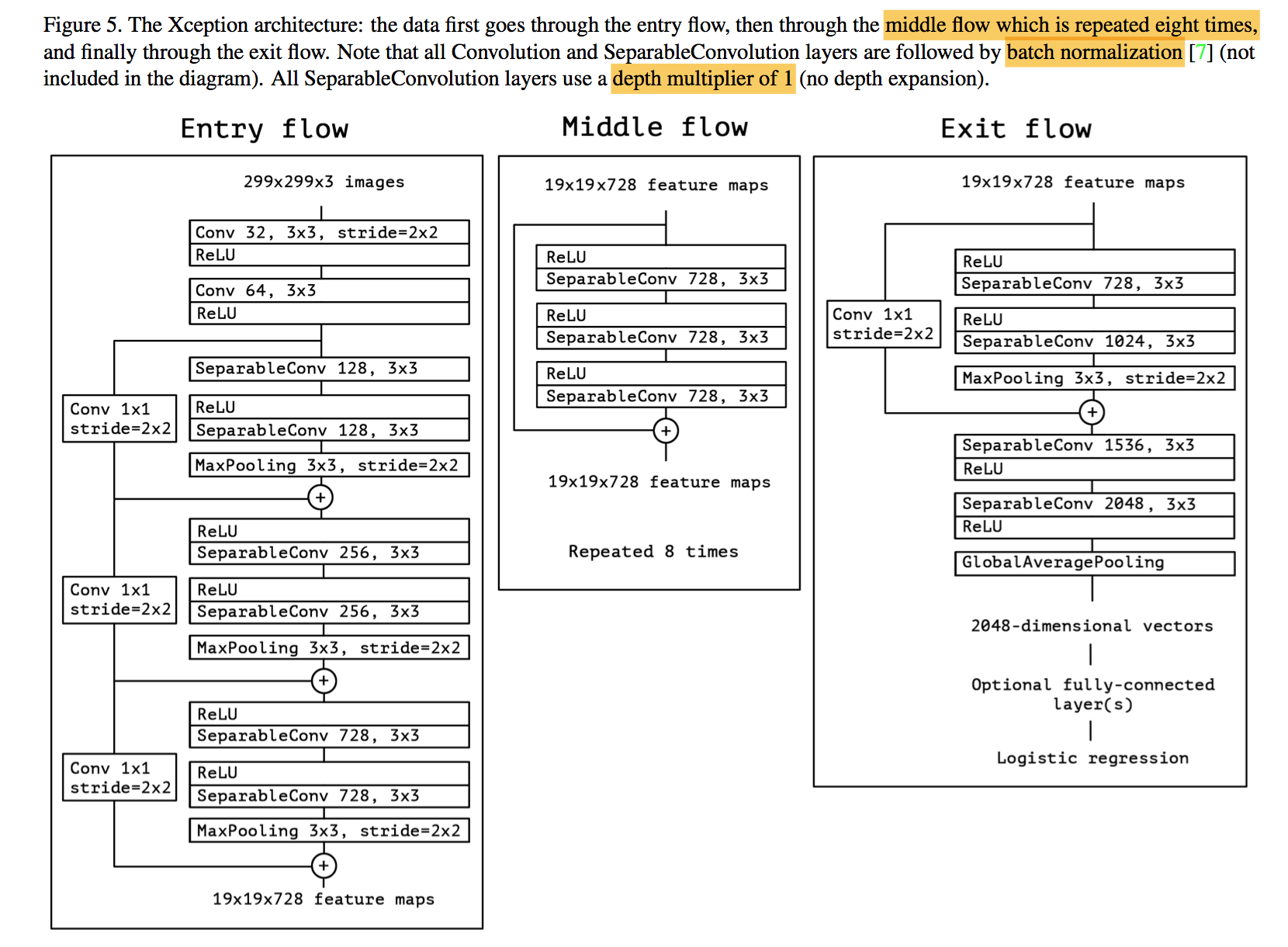
architecture
- a linear stack of depthwise separable convolution layers with residual connections
- all conv are followed by BN
keras的separableConv和depthwiseConv:前者由后者加上一个pointwiseConv组成,最后有activation,中间没有
cmp
- Xception and Inception V3 have nearly the same number of parameters
- marginally better on ImageNet
- much larger performance increasement on JFT
- Residual connections are clearly essential in helping with convergence, both in terms of speed and final classification performance.
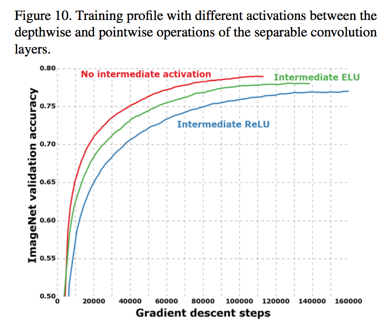
Effect of intermediate activation:the absence of any non-linearity leads to both faster convergence and better final performance
EfficientNet: Rethinking Model Scaling for Convolutional Neural Networks
动机
- common sense:scaled up the network for better accuracy
- we systematically study model scaling
- and identify that carefully balancing network depth, width, and resolution can lead to better performance
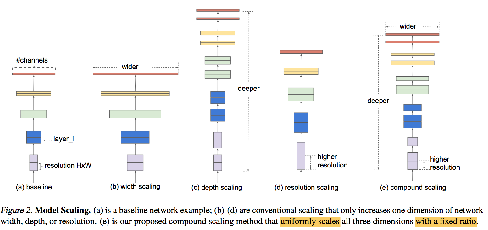
- propose a new scaling method:using compound coefficient to uniformly scale all dimensions of depth/width/resolution
- on MobileNets and ResNet
- a new baseline network family EfficientNets
- much better accuracy and efficiency
论点
- previous work scale up one of the three dimensions
- depth:more layers
- width:more channels
- image resolution:higher resolution
- arbitrary scaling requires tedious manual tuning and often yields sub-optimal accuracy and efficiency
uniformly scaling:Our empirical study shows that it is critical to balance all dimensions of network width/depth/resolution, and surprisingly such balance can be achieved by simply scaling each of them with constant ratio.
neural architecture search:becomes increasingly popular in designing efficient mobile-size ConvNets
- previous work scale up one of the three dimensions
方法
problem formulation
ConvNets:$N = \bigodot_{i=1…s} F_i^{L_i}(X_{
simplify the design problem
- fixing $F_i$
- all layers must be scaled uniformly with constant ratio
an optimization problem:d for depth coefficients, w for width coefficients, r for resolution coefficients
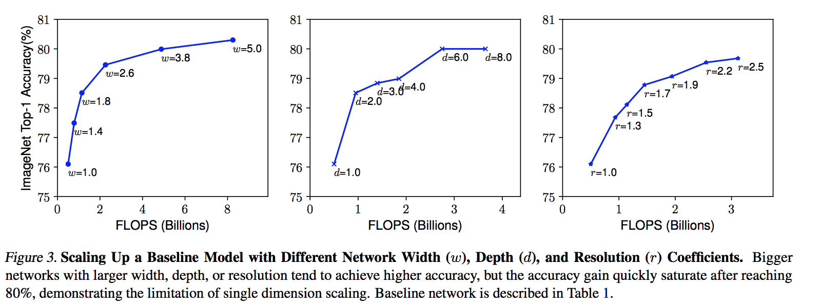
observation 1
- Scaling up any dimension of network (width, depth, or resolution) improves accuracy, but the accuracy gain diminishes for bigger models. 准确率都会提升,最终都会饱和
- depth:deeper ConvNet can capture richer and more complex features
- width:wider networks tend to be able to capture more fine-grained features and are easier to train (commonly used for small size models)但是深度和宽度最好匹配,一味加宽shallow network会较难提取高级特征
- resolution:higher resolution input can potentially capture more fine-grained patterns
observation 2
compound scaling:it is critical to balance all dimensions of network width, depth, and resolution
different scaling dimensions are not independent 输入更高的resolution,就需要更深的网络,以获取更大的感受野,同时还需要更宽的网络,以捕获更多的细粒度特征
compound coefficient $\phi$:
- $\alpha, \beta, \gamma$ are constants determined by a small grid search, controling the assign among the 3 dimensions [d,w,r]
- $\phi$ controls how many more resources are available for model scaling
- the total FLOPS will approximately increase by $2^\phi$
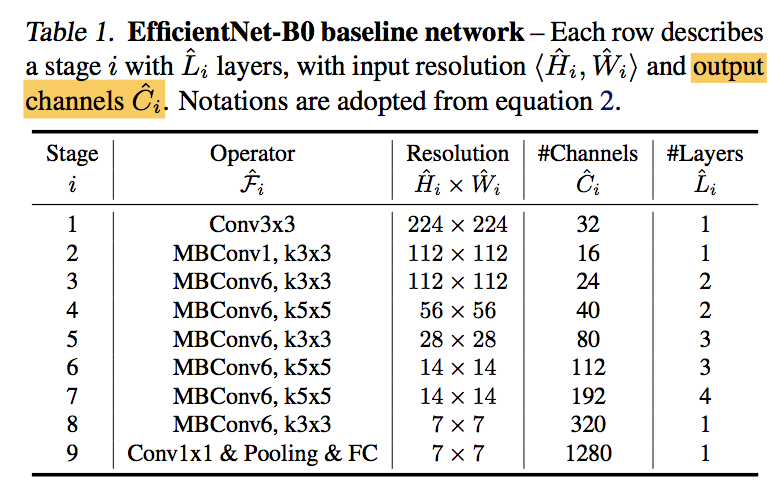
efficientNet architecture
having a good baseline network is also critical
thus we developed a new mobile-size baseline called EfficientNet by leveraging a multi-objective neural architecture search that optimizes both accuracy and FLOPS
compound scaling:fix $\phi=1$ and grid search $\alpha, \beta, \gamma$, fix $\alpha, \beta, \gamma$ and use different $\phi$
实验
on MobileNets and ResNets
- compared to other single-dimension scaling methods
- compound scaling method improves the accuracy on all
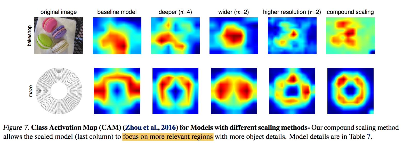
on EfficientNet
- model with compound scaling tends to focus on more relevant regions with more object details
while other models are either lack of object details or unable to capture all objects in the images
implementing details
- RMSProp: decay=0.9, momentum(rho)=0.9,tpu上使用lars
- BN: momentum=0.99
- weight decay = 1e-5
- lr: initial=0.256, decays by 0.97 every 2.4 epochs
- SiLU activation
- AutoAugment
- Stochastic depth: survive_prob = 0.8
- dropout rate: 0.2 to 0.5 for B0 to B7
EfficientDet: Scalable and Efficient Object Detection
动机
- model efficiency
- for object detection:based on one-stage detector
- 特征融合:propose a weighted bi-directional feature pyramid network (BiFPN)
- 网络rescale:uniformly scales the resolution, depth, and width for all backbone
- achieve better accuracy with much fewer parameters and FLOPs
- also test on Pascal VOC 2012 semantic segmentation
论点
- previous work tends to achieve better efficiency by sacrificing accuracy
- previous work fuse feature at different resolutions by simply summing up without distinction
- EfficientNet
- backbone:combine EfficientNet backbones with our propose BiFPN
- scale up:jointly scales up the resolution/depth/width for all backbone, feature network, box/class prediction network
- Existing object detectors
- two-stage:have a region-of-interest proposal step
- one-stage:have not, use predefined anchors
方法
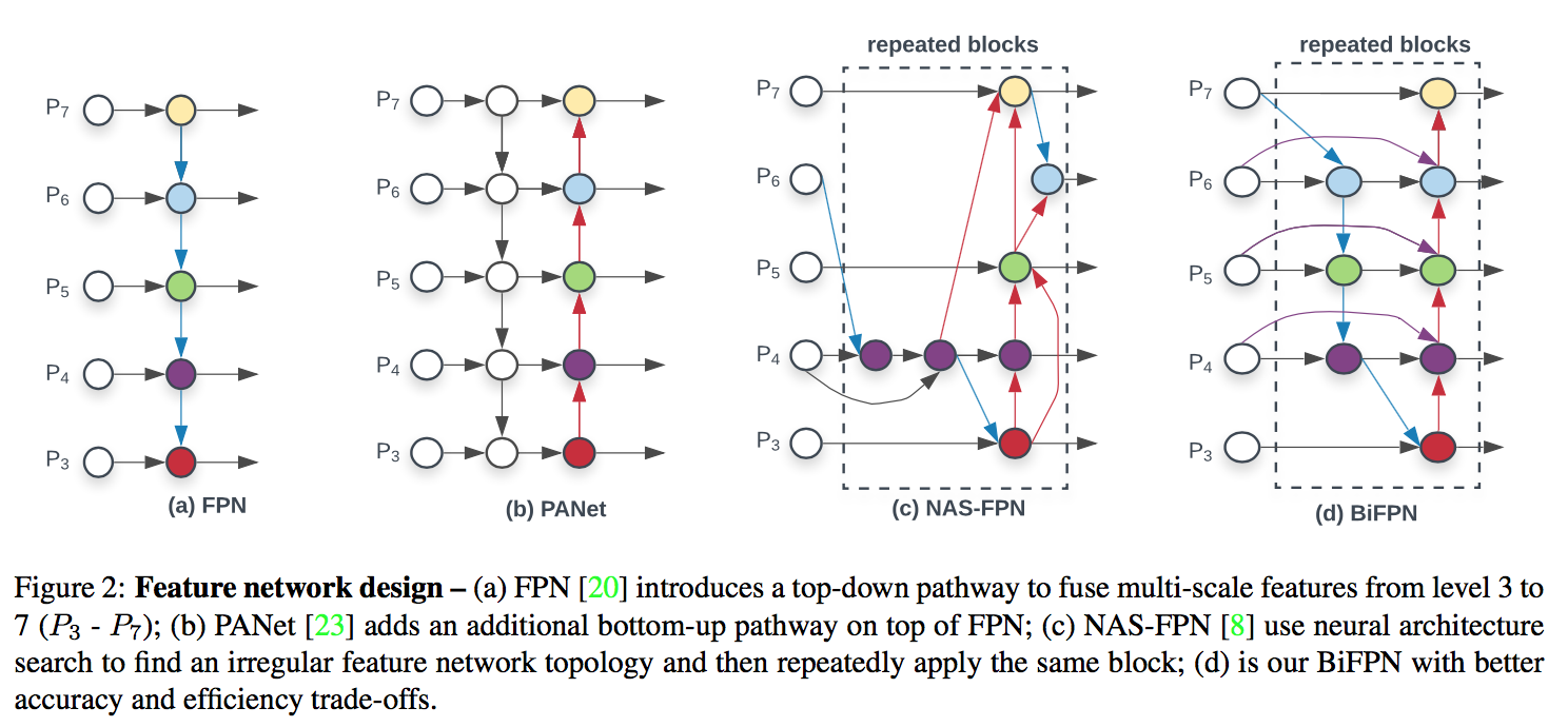
BiFPN:efficient bidirectional cross-scale connec- tions and weighted feature fusion
FPN:limit是只有top-bottom一条information flow
PANet:加上了一条bottom-up path,better accuracy但是more parameters and computations
NAS-FPN:基于网络搜索出的结构,irregular and difficult to interpret or modify
BiFPN
- remove those nodes that only have one input edge:只有一条输入的节点,没做到信息融合
- add an extra edge from the original input to output node if they are at the same level:fuse more features without adding much cost
repeat blocks
Weighted Feature Fusion
- since different input features are at different resolutions, they usually contribute to the output feature unequally
- learnable weight that can be a scalar (per-feature), a vector (per-channel), or a multi-dimensional tensor (per-pixel)
weight normalization
- Softmax-based:$O=\sum_i \frac{e^{w_i}}{\sum_j e^{w_j}}*I_i$
- Fast normalized:$O=\sum_i \frac{w_i}{\epsilon + \sum_j w_j}*I_i$,Relu is applied after each $w_i$ to keep non-negative
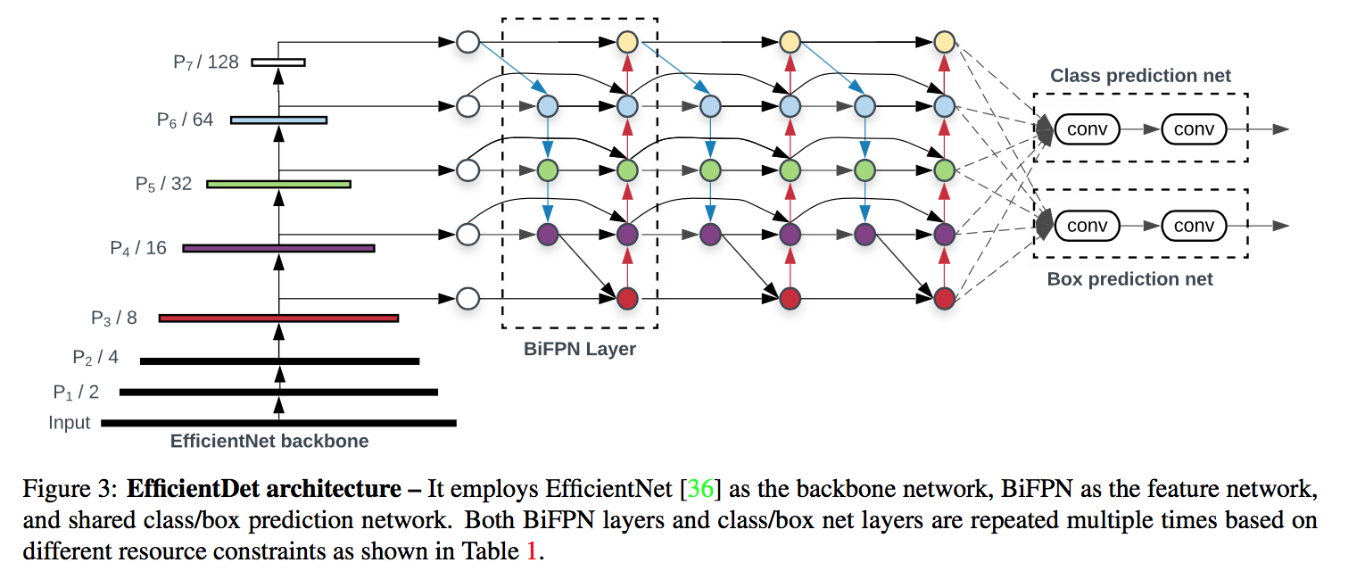
EfficientDet
- ImageNet-pretrained Effi- cientNets as the backbone
- BiFPN serves as the feature network
the fused features(level 3-7) are fed to a class and box network respectively
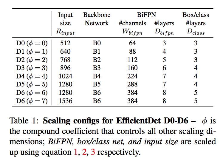
compound scaling
backbone:reuse the same width/depth scaling coefficients of EfficientNet-B0 to B6
feature network:
- depth(layers):$D=3+\phi$
- width(channes):$W=64 \cdot (1.35^{\phi}) $
box/class prediction network:
- depth:$D=3+[\phi/3]$
- width:same as FPN
resolution
- use feature 3-7:must be dividable by $2^7$
- $R=512+128*\phi$
EfficientDet-D0 ($\phi=0$) to D7 ($\phi=7$)
实验
- for object detection
- train
- Learning rate is linearly increased from 0 to 0.16 in the first training epoch and then annealed down
- employ commonly-used focal loss
- 3x3 anchors
- compare
- low-accuracy regime:低精度下,EfficientDet-D0和yoloV3差不多
- 中等精度,EfficientDet-D1和Mask-RCNN差不多
- EfficientDet-D7 achieves a new state-of-the-art
- train
- for semantic segmentation
- modify
- keep feature level {P2,P3,…,P7} in BiFPN
- but only use P2 for the final per-pixel classification
- set the channel size to 128 for BiFPN and 256 for classification head
- Both BiFPN and classification head are repeated by 3 times
- compare
- 和deeplabv3比的,COCO数据集
- better accuracy and fewer FLOPs
- modify
- ablation study
- backbone improves accuracy v.s. resnet50
- BiFPN improves accuracy v.s. FPN
- BiFPN achieves similar accuracy as repeated FPN+PANet
- BiFPN + weghting achieves the best accuracy
- Normalized:softmax和fast版本效果差不多,每个节点的weight在训练开始迅速变化(suggesting different features contribute to the feature fusion unequally)
- Compound Scaling:这个比其他只提高一个指标的效果好就不用说了
- for object detection
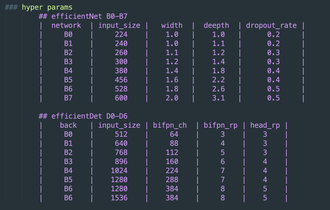
超参:
efficientNet和efficientDet的resolution是不一样的,因为检测还有neck和head,层数更深,所以resolution更大
EfficientNetV2: Smaller Models and Faster Training
动机
- faster training speed and better parameter efficiency
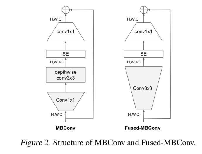
- use a new op: Fused-MBConv
- propose progressive learning:adaptively adjuts regularization & image size
方法
review of EfficientNet
large image size
- large memory usage,small batch size,long training time
- thus propose increasing image size gradually in V2
extensive depthwise conv
- often cannot fully utilize modern accelerators
thus introduce Fused-MBConv in V2:When applied in early stage 1-3, Fused-MBConv can improve training speed with a small overhead on parameters and FLOPs
equally scaling up
- proved sub-optimal in nfnets
- since the stages are not equally contributed to the efficiency & accuracy
- thus in V2
- use a non-uniform scaling strategy:gradually add more layers to later stages(s5 & s6)
- restrict the max image size
EfficientNet V2 Architecture
basic ConvBlock
- use fused-MBConv in the early layers
- use MBConv in the latter layers
expansion ratios
- use smaller expansion ratios
- 因为同样的通道数,fused-MB比MB的参数量大
kernel size
- 全图3x3,没有5x5了
- add more layers to compensate the reduced receptive field
last stride 1 stage
- effv1是7个stage
effv2有6个stage
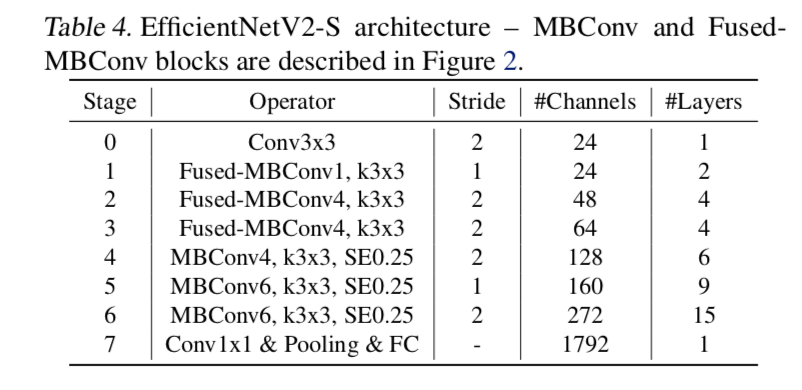
scaling policy
- compound scaling:R、W、D一起scale
- 但是限制了最大inference image size=480(train=384)
- gradually add more layers to later stages (s5 & s6)
progressive learning
large models require stronger regularization
larger image size leads to more computations with larger capacity,thus also needs stronger regularization
training process
- in the early training epochs, we train the network with smaller images and weak regularization
gradually increase image size but also making learning more difficult by adding stronger regularization
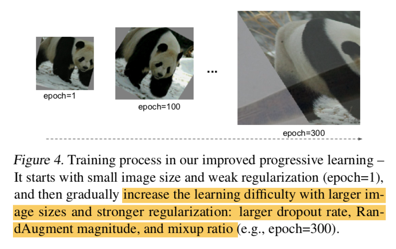
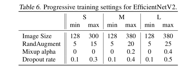
adaptive params
- image size
- dropout rate
- randAug magnitude
- mixup alpha
给定最大最小值,stage N,使用linear interpolation
train&test details
- RMSProp optimizer with decay 0.9 and momentum 0.9
- batch norm momentum 0.99
- weight decay 1e-5
- trained for 350 epochs with total batch size 4096
- Learning rate is first warmed up from 0 to 0.256, and then decayed by 0.97 every 2.4 epochs
- exponential moving average with 0.9999 decay rate
stochastic depth with 0.8 survival probability
4 stages (87 epochs per stage):early stage with weak regularization & later stronger
- maximum image size for training is about 20% smaller than inference & no further finetuning