FCN: Fully Convolutional Networks for Semantic Segmentation
动机
- take input of arbitrary size
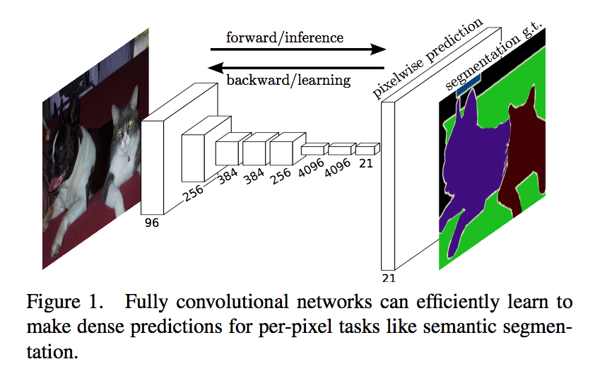
- pixelwise prediction (semantic segmentation)
- efficient inference and learning
- end-to-end
- with superwised-pretraining
论点
- fully connected layers brings heavy computation
- patchwise/proposals training with less efficiency (为了对一个像素分类,要扣它周围的patch,一张图的存储容量上升到k*k倍,而且相邻patch重叠的部分引入大量重复计算,同时感受野太小,没法有效利用全局信息)
- fully convolutional structure are used to get a feature extractor which yield a localized, fixed-length feature
- Semantic segmentation faces an inherent tension between semantics and location: global information resolves what while local information resolves where. Deep feature hierarchies jointly encode location and semantics in a local-to-global pyramid.
- other semantic works (RCNN) are not end-to-end
要素
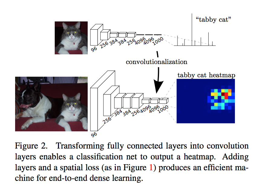
- 把全连接层换成1*1卷积,用于提取特征,形成热点图
- 反卷积将小尺寸的热点图上采样到原尺寸的语义分割图像
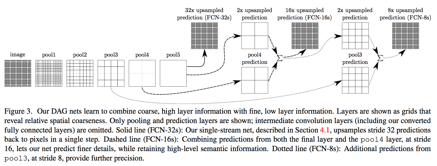
- a novel “skip” architecture to combine deep, coarse, semantic information and shallow, fine, appearance information
方法
fully convolutional network
- receptive fields: Locations in higher layers correspond to the locations in the image they are path-connected to
- typical recognition nets:
- fixed-input
- patches
- the fully connected layers can be viewed as convolutions with kernels that cover their entire input regions
- our structure:
- arbitrary-input
- the computation is saved by computing the overlapping regions of those patches only once
- output size corresponds to the input(H/16, W/16)
- heatmap: the (H/16 * W/16) high-dims feature-map corresponds to the 1000 classes
-
- OverFeat introduced
- 对于高维特征图上一个元素,对应了原图感受野一片区域,将reception field中c位填上这个元素的值
- 移动原图,相应的感受野对应的图片也发生了移动,高维特征图的输出变了,c位变了
- 移动范围stride*stride,就会得到原图尺寸的输出了
upsampling
- simplest: bilinear interpolation
- in-network upsampling: backwards convolution (deconvolution) with an output stride of f
- A stack of deconvolution layers and activation functions can even learn a nonlinear upsampling
- factor: FCN里面inputsize和outputsize之间存在线性关系,就是所有卷积pooling层的累积采样步长乘积
- kernelsize:$2 * factor - factor \% 2$
- stride:$factor$
- padding:$ceil((factor - 1) / 2.)$
这块的计算有点绕,$stride=factor$比较好确定,这是将特征图恢复的原图尺寸要rescale的尺度。然后在输入的相邻元素之间插入s-1个0元素,原图尺寸变为$(s-1)(input_size-1)+input_size = sinput_size + (s-1)$,为了得到$output_size=s*input_size$输出,再至少$padding=[(s-1)/2]_{ceil}$,然后根据:
有:
在keras里面可以调用库函数Conv2DTranspose来实现:
1
2
3
4
5
6
7
8
9
10
11
12
13
14
15
16
17
18
19
20
21
x = Input(shape=(64,64,16))
y = Conv2DTranspose(filters=16, kernel_size=20, strides=8, padding='same')(x)
model = Model(x, y)
model.summary()
# input: (None, 64, 64, 16) output: (None, 512, 512, 16) params: 102,416
x = Input(shape=(32,32,16))
y = Conv2DTranspose(filters=16, kernel_size=48, strides=16, padding='same')(x)
# input: (None, 32, 32, 16) output: (None, 512, 512, 16) params: 589,840
x = Input(shape=(16,16,16))
y = Conv2DTranspose(filters=16, kernel_size=80, strides=32, padding='same')(x)
# input: (None, 16, 16, 16) output: (None, 512, 512, 16) params: 1,638,416
# 参数参考:orig unet的total参数量为36,605,042
# 各级transpose的参数量为:
# (None, 16, 16, 512) 4,194,816
# (None, 32, 32, 512) 4,194,816
# (None, 64, 64, 256) 1,048,832
# (None, 128, 128, 128) 262,272
# (None, 256, 256, 32) 16,416可以看到kernel_size变大,对参数量的影响极大。(kernel_size设置的小了,只能提取到单个元素,我觉得kernel_size至少要大于stride)
Segmentation Architecture
- use pre-trained model
- convert all fully connected layers to convolutions
- append a 1*1 conv with channel dimension(including background) to predict scores
- followed by a deconvolution layer to upsample the coarse outputs to dense outputs
skips
- the 32 pixel stride at the final prediction layer limits the scale of detail in the upsampled output
- 逐层upsampling,融合前几层的feature map,element-wise add
finer layers: “As they see fewer pixels, the finer scale predictions should need fewer layers.” 这是针对前面的卷积网络来说,随着网络加深,特征图上的感受野变大,就需要更多的channel来记录更多的低级特征组合
- add a 1*1 conv on top of pool4 (zero-initialized)
- adding a 2x upsampling layer on top of conv7 (We initialize this 2xupsampling to bilinear interpolation, but allow the parameters to be learned)
- sum the above two stride16 predictions (“Max fusion made learning difficult due to gradient switching”)
- 16x upsampled back to the image
做到第三行再往下,结果又会变差,所以做到这里就停下
总结
在升采样过程中,分阶段增大比一步到位效果更好
在升采样的每个阶段,使用降采样对应层的特征进行辅助
8倍上采样虽然比32倍的效果好了很多,但是结果还是比较模糊和平滑,对图像中的细节不敏感,许多研究者采用MRF算法或CRF算法对FCN的输出结果做进一步优化
x8为啥好于x32:1. x32的特征图感受野过大,对小物体不敏感 2. x32的放大比例造成的失真更大
unet的区别:
unet没用imagenet的预训练模型,因为是医学图像
unet在进行浅层特征融合的时候用了concat而非element-wise add
逐层上采样,x2 vs. x8/x32
orig unet没用pad,输出小于输入,FCN则pad+crop
数据增强,FCN没用这些‘machinery’,医学图像需要强augmentation
加权loss