U-NET: Convolutional Networks for Biomedical Image Segmentation
动机:
- train from very few images
- outperforms more precisely on segmentation tasks
- fast
要素:
- 编码:a contracting path to capture context
- 解码:a symmetric expanding path that enables precise localization
- 实现:pooling operators & upsampling operators
论点:
when we talk about deep convolutional networks:
- larger and deeper
- millions of parameters
- millions of training samples
representative method:run a sliding-window and predict a pixel label based on its‘ patch
- drawbacks:
- calculating redundancy of overlapping patches
- big patch:more max-pooling layers that reduce the localization accuracy
- small patch:less involvement of context
- metioned but not further explained:cascade structure
方法:
In order to localize, high resolution features from the contracting path are combined with the upsampled output. A successive convolution layer can then learn to assemble a more precise output based on this information.
理解:深层特征层感受野较大,带有全局信息,将其上采样用于提供localization information,而横向add过来特征层带有局部特征信息。两个3*3的conv block用于将两类信息整合,输出更精确的表达。
In the upsampling part we have also a large number of feature channels, which allow the network to propagate context information to higher resolution layers.
理解:应该是字面意思吧,为上采样的卷积层保留更多的特征通道,就相当于保留了更多的上下文信息。
we use excessive data augmentation.
细节:
contracting path:
- typical CNN:blocks of [2 3*3 unpadded convs+ReLU+2*2 stride2 maxpooling]
- At each downsampling step we double the number of feature channels
expansive path:
- upsampling:
- 2*2 up-conv that half the channels
- concatenation the corresponding cropped feature map from the contracting path
- 2 [3x3 conv+ReLU]
- final layer:use a 1*1 conv to map the feature vectors to class vectors
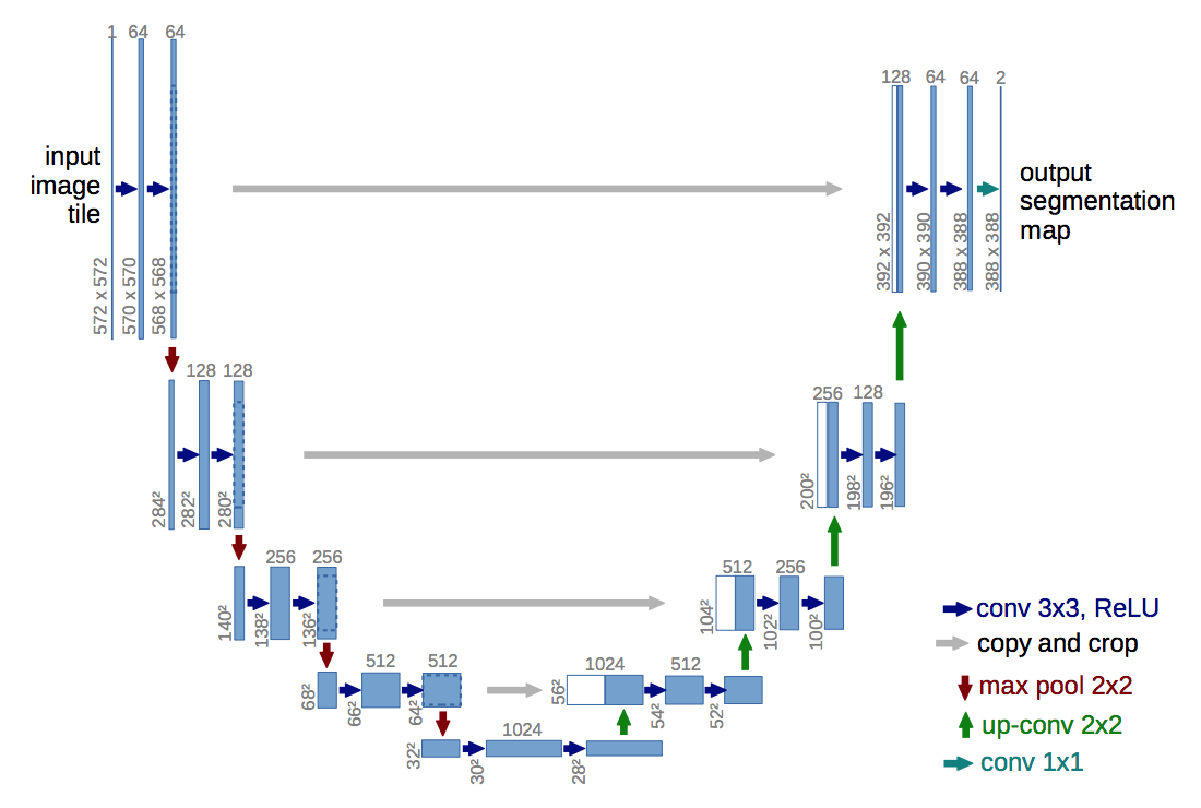
- upsampling:
train:
- prefer larger input size to larger batch size
- sgd with 0.99 momentum so that the previously seen samples dominate the optimization
loss:softmax & cross entropy
unbalanced weight:
- pre-compute the weight map base on the frequency of pixels for a certain class
- add the weight for a certain element to force the learning emphasis:e.g. the small separation borders
- initialization:Gaussian distribution
data augmentation:
- deformations
- “Drop-out layers at the end of the contracting path perform further implicit data augmentation”
metrics:“warping error”, the “Rand error” and the “pixel error” for EM segmentation challenge and average IOU for ISBI cell tracking challenge
prediction:
按照论文的模型结构,输入和输出的维度是不一样的——在valid padding的过程中有边缘信息损失。
那么如果我们想要预测黄框内的分割结果,需要输入一张更大的图(蓝框)作为输入,在图片边缘的时候,我们通过镜像的方式补全。
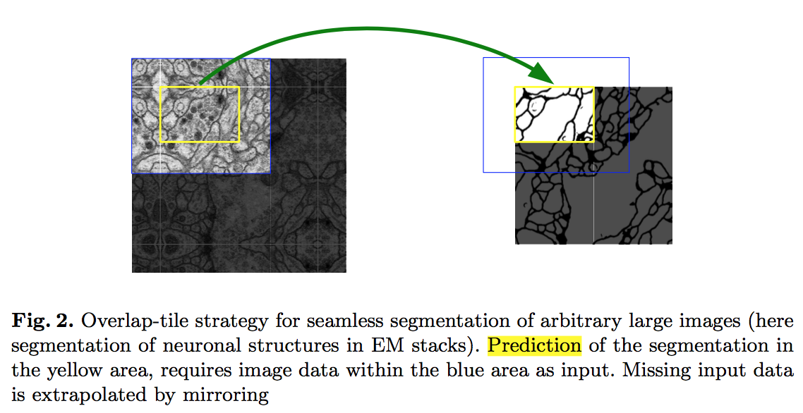
因果关系:
- 首先因为内存限制,输入的不是整张图,是图片patch,
- 为了保留上下文信息,使得预测更准确,我们给图片patch添加一圈border的上下文信息(实际感兴趣的是黄框区域)
- 在训练时,为了避免重叠引入的计算,卷积层使用了valid padding
- 因此在网络的输出层,输出尺寸才是我们真正关注的部分
- 如果训练样本尺寸不那么huge,完全可以全图输入,然后使用same padding,直接预测全图mask
总结:
- train from very few images —-> data augmentation
- fast —-> full convolution layers
- precise —-> global?
V-Net: Fully Convolutional Neural Networks for Volumetric Medical Image Segmentation
动机
- entire 3D volume
- imbalance between the number of foreground and background voxels:dice coefficient
- limited data:apply random non-linear transformations and histogram matching
- fast and accurate
论点:
- early approaches based on patches
- local context
- challenging modailities
- efficiency issues
- fully convolutional networks
- 2D so far
- imbalance issue:the anatomy of interest occupies only a very small region of the scan thus predictions are strongly biased towards the background.
- re-weighting
- dice coefficient claims to be better that above
- early approaches based on patches
要素:
- a compression path
a decompression path
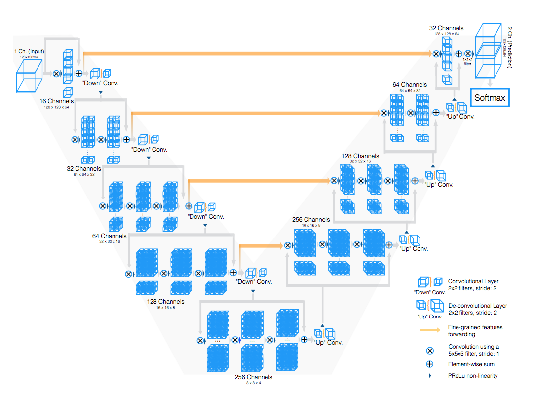
方法:
compression:
- add residual能够加速收敛
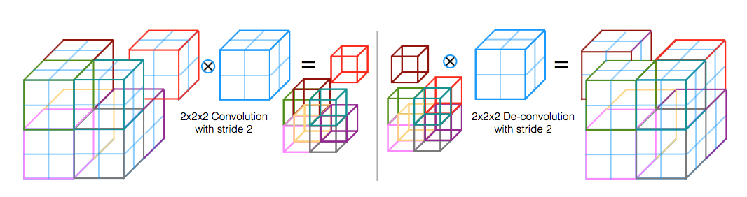
- resolution is reduced by [2*2*2 conv with stride 2]相比于maxpooling节省了bp所需switch map的memory消耗
- double the number of feature maps as we reduce their resolution
- PReLU
decompression:
- horizontal connections:1) gather fine grained detail that would be otherwise lost in the compression path 2) improve the convergence time
residual conv:blocks of [5*5*5 conv with stride 1] 提取特征继续增大感受野
up-conv:expands the spatial support of the lower resolution feature maps
last layer:run [1*1*1conv with 2 channel+softmax] to obtain the voxelwise probabilistic segmentations of the foreground and background
dice coefficient: [0,1] which we aim to maximise,assume $p_i$、$g_i$ belong to two binary volumes
train:
- input fix size 128 × 128 × 64 voxels and a spatial resolution of 1 × 1 × 1.5 millimeters
- each mini-batch contains 2 volumes
- online augmentation:
- randomly deformation
- vary the intensity distribution:随机选取样本的灰度分布作为当前训练样本的灰度分布
- used a momentum of 0.99 and a initial learning rate of 0.0001 which decreases by one order of magnitude every 25K iterations
metrics:
- Dice coefficient
- Hausdorff distance of the predicted delineation to the ground truth annotation
- the score obtained on the challenge
dice loss & focal loss
CE & BCE
CE:categorical_crossentropy,针对所有类别计算,类别间互斥
$x$是输入样本,$y_i$是第$i$个类别对应的真实标签,$f_i(x)$是对应的模型输出值。
对分类问题,$y_i$是one-hot,$f_i(x)$是个一维向量。最终得到一个数值。
BCE:binary_crossentropy,针对每个类别计算
$i$是类别编号,最终得到一个维度为$n_class$的向量。
再求类均值得到一个数值作为单个样本的loss。
batch loss:对batch中所有样本的loss求均值。
从公式上看,CE的输出通常是经过了softmax,softmax的某一个输出增大,必然导致其它类别的输出减小,因此在计算loss的时候关注正确类别的预测值是否被拉高即可。使用BCE的场景通常是使用sigmoid,类别间不会互相压制,因此既要考虑所属类别的预测概率够高,也要考虑不所属类别的预测概率足够低(这一项在softmax中被实现了故CE不需要这一项)。
- 场景:
- 二分类:只有一个输出节点,$f(x) \in (0,1)$,应该使用sigmoid+BCE作为最后的输出层配置。
- 单标签多分类:应该使用softmax+CE的方案,BCE也同样适用。
- 多标签多分类:multi-label每个标签的输出是相互独立的,因此常用配置是sigmoid+BCE。
- 对分割场景来说,输出的每一个channel对应一个类别的预测map,可以看成是多个channel间的单标签多分类(softmax+CE),也可以看成是每个独立通道类别map的二分类(sigmoid+BCE)。unet论文用了weighted的softmax+CE。vnet论文用了dice_loss。
re-weighting(WCE)
基于CE&BCE,给了样本不同的权重。
unet论文中提到了基于pixel frequency为不同的类别创建了weight map。
一种实现:基于每个类别的weight map,在实现CE的时候改成加权平均即可。
另一种实现:基于每个样本的weight map,作为网络的附加输入,在实现CE的时候乘在loss map上。
focal loss
提出是在目标检测领域,用于解决正负样本比例严重失调的问题。
也是一种加权,但是相比较于re-weighting,困难样本的权重由网络自行推断出,通过添加$(\alpha)$和$(-)^\lambda$这一加权项:
对于类别间不均衡的情况(通常负样本远远多于正样本),$(\alpha)$项用于平衡正负样本权重。
对于类内困难样本的挖掘,$(-)^\lambda$项用于调整简单样本和困难样本的权重,预测概率更接近真实label的样本(简单样本)的权重会衰减更快,预测概率比较不准确的样本(苦难样本)的权重则更高些。
由于分割网络的输出的单通道/多通道的图片,直接使用focal loss会导致loss值很大。
1. 通常与其他loss加权组合使用
2. sum可以改成mean
3.不建议在训练初期就加入,可在训练后期用于优化模型
4. 公式中含log计算,可能导致nan,要对log中的元素clip
1
2
3
4
5
6
7
8
9
10
11
12
13
def focal_loss(y_true, y_pred):
gamma = 2.
alpha = 0.25
# score = alpha * y_true * K.pow(1 - y_pred, gamma) * K.log(y_pred) + # this works when y_true==1
# (1 - alpha) * (1 - y_true) * K.pow(y_pred, gamma) * K.log(1 - y_pred) # this works when y_true==0
pt_1 = tf.where(tf.equal(y_true, 1), y_pred, tf.ones_like(y_pred))
pt_0 = tf.where(tf.equal(y_true, 0), y_pred, tf.zeros_like(y_pred))
# avoid nan
pt_1 = K.clip(pt_1, 1e-3, .999)
pt_0 = K.clip(pt_0, 1e-3, .999)
score = -K.sum(alpha * K.pow(1. - pt_1, gamma) * K.log(pt_1)) - \
K.sum((1 - alpha) * K.pow(pt_0, gamma) * K.log(1. - pt_0))
return score
dice loss
dice定义两个mask的相似程度:
- 分子是TP——只关注前景
分母可以是$|A|$(逐个元素相加),也可以是平方形式$|A|^2$
梯度:“使用dice loss有时会不可信,原因是对于softmax或log loss其梯度简言之是p-t ,t为目标值,p为预测值。而dice loss 为 2t2 / (p+t)2
如果p,t过小会导致梯度变化剧烈,导致训练困难。”
【详细解释下】交叉熵loss:$L=-(1-|t-p|)log(1-|t-p|)$,求导得到$\frac{\partial L}{\partial p}=-log(1-|t-p|)$,其实就可以简化看作$t-p$,很显然这个梯度是有界的,因此使用交叉熵loss的优化过程比较稳定。而dice loss的两种形式(不平方&平方):$L=\frac{2pt}{p+t}\ or\ L=\frac{2pt}{p^2+t^2}$,求导以后分别是$\frac{\partial L}{\partial p} = \frac{t^2+2pt}{(p+t)^2} \ or\ \frac{3tp^2+t^3}{(p^2+t^2)^2}$计算结果比较复杂,pt都很小的情况下,梯度值可能很大,可能导致训练不稳定,loss曲线混乱。
vnet论文中的定义在分母上稍有不同(see below)。smoothing的好处:
- 避免分子除0
减少过拟合
1
2
3
4
5
6
7
8
def dice_coef(y_true, y_pred):
smooth = 1.
intersection = K.sum(y_true * y_pred, axis=[1,2,3])
union = K.sum(y_true, axis=[1,2,3]) + K.sum(y_pred, axis=[1,2,3])
return K.mean( (2. * intersection + smooth) / (union + smooth), axis=0)
def dice_coef_loss(y_true, y_pred):
1 - dice_coef(y_true, y_pred, smooth=1)
iou loss
dice loss衍生,intersection over union:
分母上比dice少了一个intersection。
- “IOU loss的缺点同DICE loss,训练曲线可能并不可信,训练的过程也可能并不稳定,有时不如使用softmax loss等的曲线有直观性,通常而言softmax loss得到的loss下降曲线较为平滑。”
boundary loss
dice loss和iou loss是基于区域面积匹配度去学习,我们也可以使用边界匹配度去监督网络的学习。
只对边界上的像素进行评估,和GT的边界吻合则为0,不吻合的点,根据其距离边界的距离评估它的Loss。
Hausdorff distance
用于度量两个点集之间的相似程度,denote 点集$A\{a_1, a_2, …, a_p\}$,点集$B\{b_1, b_2, …, b_p\}$:
其中HD(A,B)是Hausdorff distance的基本形式,称为双向距离
hd(A,B)描述的是单向距离,首先找到点集A中每个点在点集B中距离最近的点作为匹配点,然后计算这些a-b-pair的距离的最大值。
HD(A,B)取单向距离中的最大值,描述了两个点集合的最大不匹配程度。
mix loss
- BCE + dice loss:在数据较为平衡的情况下有改善作用,但是在数据极度不均衡的情况下,交叉熵损失会在几个训练之后远小于Dice 损失,效果会损失。
- focal loss + dice loss:数量级问题
MSE
关键点检测有时候也会采用分割框架,这时候ground truth是高斯map,dice是针对二值化mask的,这时候还可以用MSE。
ohnm
online hard negative mining 困难样本挖掘
Tversky loss
一种加权的dice loss,dice loss会平等的权衡FP(精度,假阳)和FN(召回,假阴),但是医学图像中病灶数目远少于背景数量,很可能导致训练结果偏向高精度但是低召回率,Tversky loss控制loss更偏向FN:
1
2
3
4
5
6
7
8
9
10
11
def tversky_loss(y_true, y_pred):
y_true_pos = K.flatten(y_true)
y_pred_pos = K.flatten(y_pred)
# TP
true_pos = K.sum(y_true_pos * y_pred_pos)
# FN
false_neg = K.sum(y_true_pos * (1-y_pred_pos))
# FP
false_pos = K.sum((1-y_true_pos) * y_pred_pos)
alpha = 0.7
return 1 - (true_pos + K.epsilon())/(true_pos + alpha * false_neg + (1-alpha) * false_pos + K.epsilon())Lovasz hinge & Lovasz-Softmax loss
IOU loss衍生,jaccard loss只适用于离散情况,而网络预测是连续值,如果不使用某个超参将神经元输出二值化,就不可导。blabla
一些补充
改进:
- dropout、batch normalization:从论文上看,unet只在最深层卷积层后面添加了dropout layer,BN未表,而common sense用每一个conv层后面接BN层能够替换掉dropout并能获得性能提升的。
- UpSampling2D、Conv2DTranspose:unet使用了上采样,vnet使用了deconv,但是“DeConv will produce image with checkerboard effect, which can be revised by upsample and conv”(Reference)。
- valid padding、same padding:unet论文使用图像patch作为输入,特征提取时使用valid padding,损失边缘信息。
- network blocks:unet用的conv block是两个一组的3*3conv,vnet稍微不同一点,可以尝试的block有ResNet/ResNext、DenseNet、DeepLab等。
- pretrained encoder:feature extraction path使用一些现有的backbone,可以加载预训练权重(Reference),加速训练,防止过拟合。
- 加入SE模块(Reference):对每个通道的特征加权
- attention mechanisms:
- 引用nn-Unet主要结构改进合集:“Just to provide some prominent examples: variations of encoder-decoder style architectures with skip connections, first introduced by the U-Net [12], include the introduction of residual connections [9], dense connections [6], at- tention mechanisms [10], additional loss layers [5], feature recalibration [13], and others [11].
衍生:
TernausNet: U-Net with VGG11 Encoder Pre-Trained on ImageNet for Image Segmentation
nnU-Net: Breaking the Spell on Successful Medical Image Segmentation
TernausNet: U-Net with VGG11 Encoder Pre-Trained on ImageNet for Image Segmentation
动机:
- neural network initialized with pre-trained weights usually shows better performance than those trained from scratch on a small dataset.
- 保留encoder-decoder的结构,同时充分利用迁移学习的优势
论点:
- load pretrained weights
- 用huge dataset做预训练
方法:
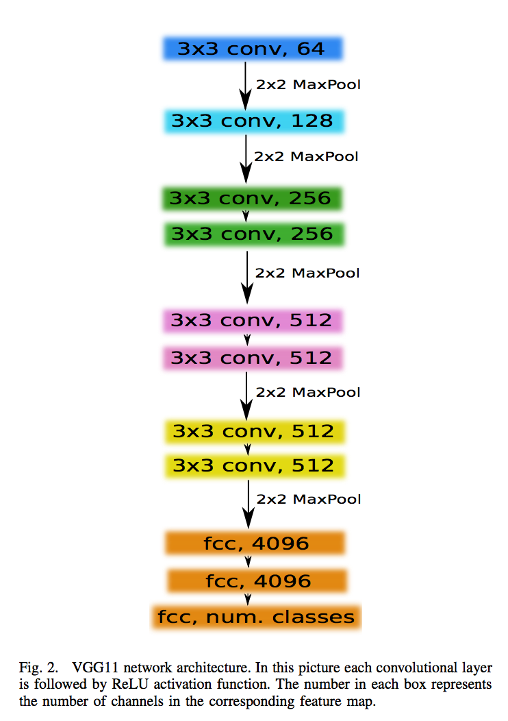
- 用vgg11替换原始的encoder,并load pre-trained weights on ImageNet:
- 最深层输入(maxpooling5):use a single conv of 512 channels that serves as a bottleneck central part of the network
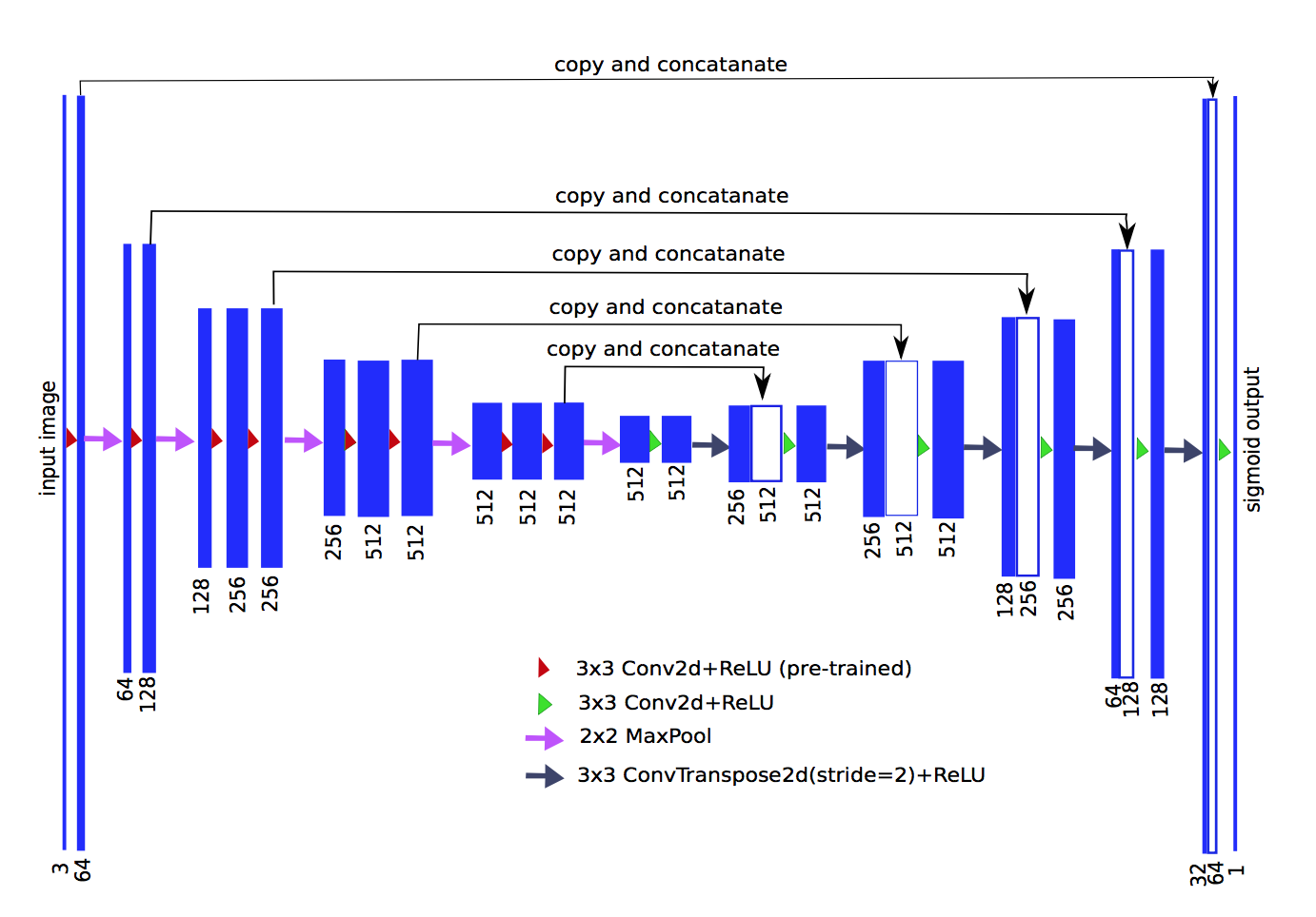
upsampling换成了convTranspose
loss function:IOU + BCE:
inference:choose a threshold 0.3, all pixel values below which are set to be zero
结论:
- converge faster
- better IOU
nnU-Net: Breaking the Spell on Successful Medical Image Segmentation
动机
- many proposed methods fail to generalize: 对于分割任务,从unet出来之后的几年里,在网络结构上已经没有多少的突破了,结构修改越多,反而越容易过拟合
- relies on just a simple U-Net architecture embedded in a robust training scheme
- automate necessary adaptations such as preprocessing, the exact patch size, batch size, and inference settings based on the properties of a given dataset: 更多的提升其实在于理解数据,针对数据采用适当的预处理和训练方法和技巧
论点
- the diversity and individual peculiarities of imaging datasets make it difficult to generalize
- prominent modifications focus on architectural modifications, merely brushing over all the other hyperparameters
- we propose: 使用基础版unet:nnUNet(no-new-Net)
- a formalism for automatic adaptation to new datasets
- automatically designs and executes a network training pipeline
- without any manual fine-tuning
要素
a segmentation task: $f_{\theta}(X) = \hat Y$, in this paper we seek for a $g(X,Y)=\theta$.
First we distinguish two type of hyperparameters:
- static params:in this case the network architecture and a robust training scheme
- dynamic params:those that need to be changed in dependence of $X$ and $Y$
Second we define g——a set of heuristics rules covering the entire process of the task:
- 预处理:resampling和normalization
- 训练:loss,optimizer设置、数据增广
- 推理:patch-based策略、test-time-augmentations集成和模型集成等
- 后处理:增强单连通域等
方法
Preprocessing
- Image Normalization:
- CT:$normed_intensity = (intensity - fg_mean) / fg_standard_deviation$, $fg$ for $[0.05,0.95]$ foreground intensity
- not CT:$normed_intensity = (intensity - mean) / standard_deviation $
- Voxel Spacing:
- for each axis chooses the median as the target spacing
- image resampled with third order spline interpolation
- z-axis using nearest neighbor interpolation if ‘anisotropic spacing’ occurs
- mask resampled with third order spline interpolation
- Image Normalization:
Training Procedure
Network Architecture:
3 independent model:a 2D U-Net, a 3D U-Net and a cascade of two 3D U-Net
padded convolutions:to achieve identical output and input shapes
instance normalization:“BN适用于判别模型,比如图片分类模型。因为BN注重对每个batch进行归一化,从而保证数据分布的一致性,而判别模型的结果正是取决于数据整体分布。但是BN对batchsize的大小比较敏感,由于每次计算均值和方差是在一个batch上,所以如果batchsize太小,则计算的均值、方差不足以代表整个数据分布;IN适用于生成模型,比如图片风格迁移。因为图片生成的结果主要依赖于某个图像实例,所以对整个batch归一化不适合图像风格化,在风格迁移中使用Instance Normalization不仅可以加速模型收敛,并且可以保持每个图像实例之间的独立。”
Leaky ReLUs
Network Hyperparameters:
- sets the batch size, patch size and number of pooling operations for each axis based on the memory consumption
- large patch sizes are favored over large batch sizes
- pooling along each axis is done until the voxel size=4
- start num of filters=30, double after each pooling
- If the selected patch size covers less than 25% of the voxels, train the 3D U-Net cascade on a downsampled version of the training data to keep sufficient context
Network Training:
- five-fold cross-validation
- One epoch is defined as processing 250 batches
- loss = dice loss + cross-entropy loss
- Adam(lr=3e-4, decay=3e-5)
- lrReduce: EMA(train_loss), 30 epoch, factor=0.2
- earlyStop: earning rate drops below 10 6 or 1000 epochs are exceeded
- data augmentation: elastic deformations, random scaling and random rotations as well as gamma augmentation($g(x,y)=f(x,y)^{gamma}$)
- keep transformations in 2D-plane if ‘anisotropic spacing’ occurs
Inference
- sliding window with half the patch size: this increases the weight of the predictions close to the center relative to the borders
- ensemble:
- U-Net configurations (2D, 3D and cascade)
- furthermore uses the five models (five-fold cross-validation)
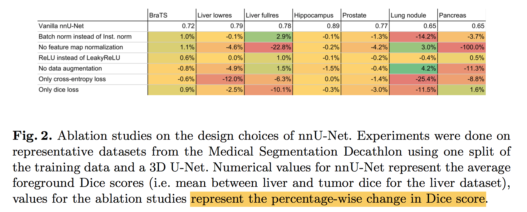
Ablation studies
3D U-Net: Learning Dense Volumetric Segmentation from Sparse Annotation
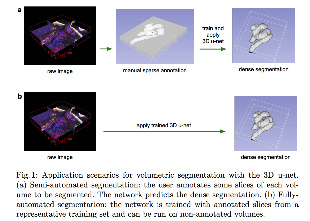
动机
- learns from sparsely/full annotated volumetric images (user annotates some slices)
- provides a dense 3D segmentation
要素
- 3D operations
- avoid bottlenecks and use batch normalization for faster convergence
- on-the-fly elastic deformation
- train from scratch
论点
- neighboring slices show almost the same information
- many biomedical applications generalizes reasonably well because medical images comprises repetitive structures
- thus we suggest dense-volume-segmentation-network that only requires some annotated 2D slices for training
scenarios
- manual annotated 一部分slice,然后训练网络实现dense seg
- 用一部分 sparsely annotated的dataset作为training set,然后训练的网络实现在新的数据集上dense seg
方法
Network Architecture
compression:2*3x3x3 convs(+BN)+relu+2x2x2 maxpooling
decompression:2x2x2 upconv+2*3x3x3 convs+relu
head:1x1x1 conv
concat shortcut connections
【QUESTION】avoid bottlenecks by doubling the number of channels already before max pooling
个人理解这个double channel是在跟原始的unet结构对比,原始unet每个stage的两个conv的filter num是一样的,然后进行max pooling会损失部分信息,但是分割任务本身是个dense prediction,所以增大channel来减少信息损失
但是不理解什么叫“avoid bottlenecks”
原文说是参考了《Rethinking the inception architecture for computer vision》大名鼎鼎的inception V3
可能对应的是“1. Avoid representational bottlenecks, especially early in the network.”,从输入到输出,要逐渐减少feature map的尺寸,同时要逐渐增加feature map的数量。
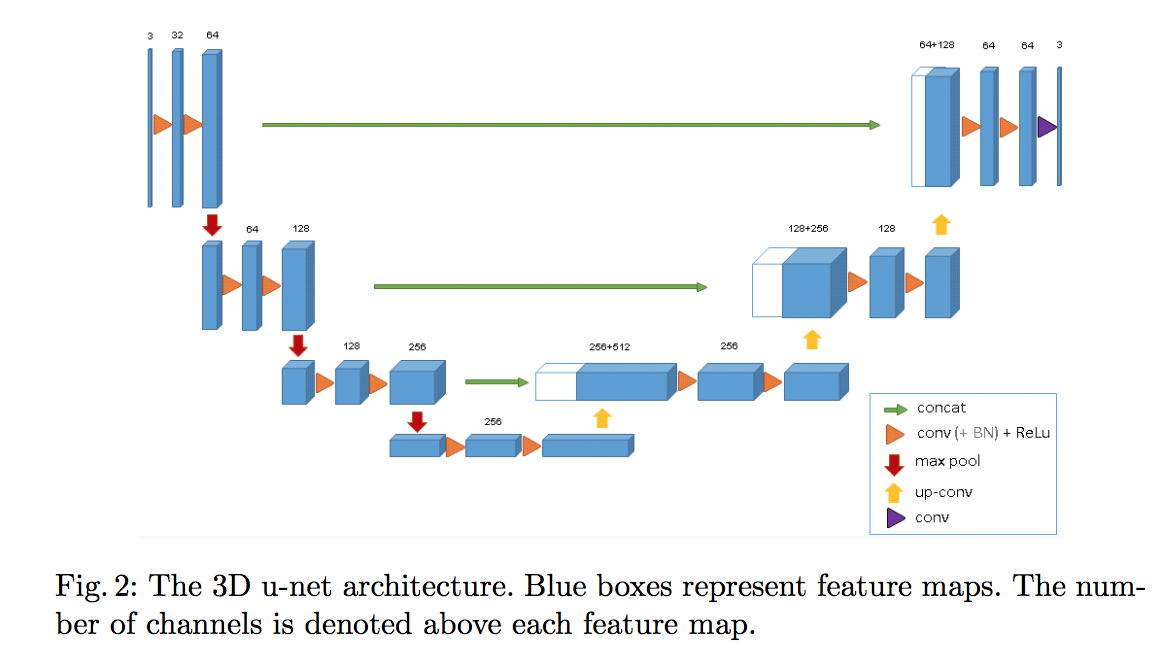
- input:132x132x116 voxel tile
- output:44x44x28
- BN:before each ReLU
weighted softmax loss function:setting the weights of unlabeled pixels to zero makes it possible to learn from only the labelled ones and, hence, to generalize to the whole volume(是不是random set the loss zeros of some samples总能让网络更好的generalize?)
Data
- manually annotated some orthogonal xy, xz, and yz slices
- annotation slices were sampled uniformly
ran on down-sampled versions of the original resolution by factor of two
labels:0: “inside the tubule”; 1: “tubule”; 2: “background”, and 3: “unlabeled”.
Training
- rotation, scaling and gray value augmentation
- a smooth dense deformation:random vector, normal distribution, B-spline interpolation
- weighted cross-entropy loss:increase weights “inside the tubule”, reduce weights “background”, set zero “unlabeled”
2.5D-UNet: Automatic Segmentation of Vestibular Schwannoma from T2-Weighted MRI by Deep Spatial Attention with Hardness-Weighted Loss
专业术语
- Vestibular Schwannoma(VS) tumors:前庭神经鞘瘤
- through-plane resolution:层厚
- isotropic resolution:各向同性
- anisotropic resolutions:各向异性
动机
tumor的精确自动分割
challenge
- low contrast:hardness-weighted Dice loss functio
- small target region:attention module
- low through-plane resolution:2.5D
论点
- segment small structures from large image contexts
- coarse-to-fine
- attention map
- Dice loss
- our method
- end-to-end supervision on the learning of attention map
- voxel-level hardness- weighted Dice loss function
- CNN
- 2D CNNs ignore inter-slice correlation
- 3D CNNs most applied to images with isotropic resolution requiring upsampling
- to balance the physical receptive field (in terms of mm rather than voxels):memory rise
- our method
- high in-plane resolution & low through-plane resolution
- 2.5D CNN combining 2D and 3D convolutions
- use inter-slice features
- more efficient than 3D CNNs
- 数据
- T2-weighted MR images of 245 patients with VS tumor
- high in-plane resolution around 0.4 mm×0.4 mm,512x512
- slice thickness and inter-slice spacing 1.5 mm,slice number 19 to 118
- cropped cube size:100 mm×50 mm×50 mm
- segment small structures from large image contexts
方法
architecture
- five levels:L1、L2 use 2D,L3、L4、L5 use 3D
- After the first two max-pooling layers that downsample the feature maps only in 2D, the feature maps in L3 and the followings have a near- isotropic 3D resolution.
- start channels:16
- conv block:conv-BN-pReLU
add a spatial attention module to each level of the decoder
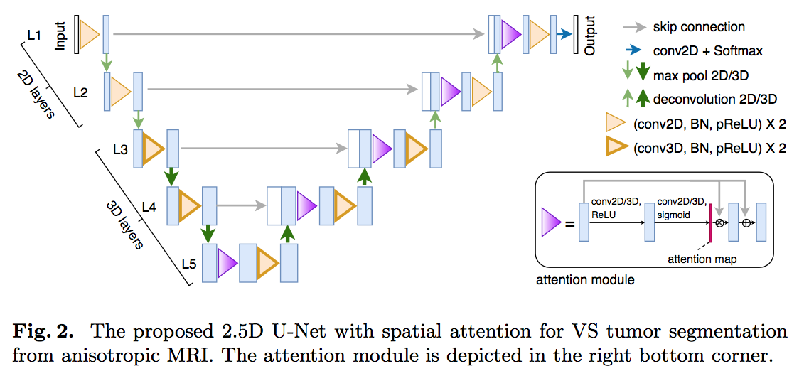
spatial attention module
- A spatial attention map can be seen as a single-channel image of attention coefficient
- input:feature map with channel $N_l$
- conv1+ReLU: channel $N_l/2$
- conv2+Sigmoid:channel 1,outputs the attention map
- multiplied the feature map with the attention map
- a residual connection
- explicit supervision
- multi-scale attention loss
- $L_{attention} = \frac{1}{L} \sum_{L} l(A_l, G_l^f)$
- $A_l$是每一层的attention map,$G_l^f$是每一层是前景ground truth average-pool到当前resolution的mask
Voxel-Level Hardness-Weighted Dice Loss
automatic hard voxel weighting:$w_i = \lambda * abs(p_i - g_i) + (1-\lambda)$
$\lambda \in [0,1]$,controls the degree of hard voxel weighting
hardness-weighted Dice loss (HDL) :
total loss:
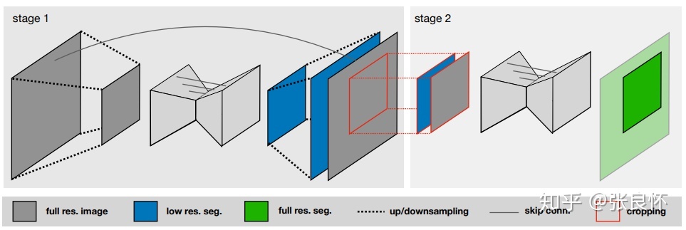
Combining analysis of multi-parametric MR images into a convolutional neural network: Precise target delineation for vestibular schwannoma treatment planning
只有摘要和一幅图
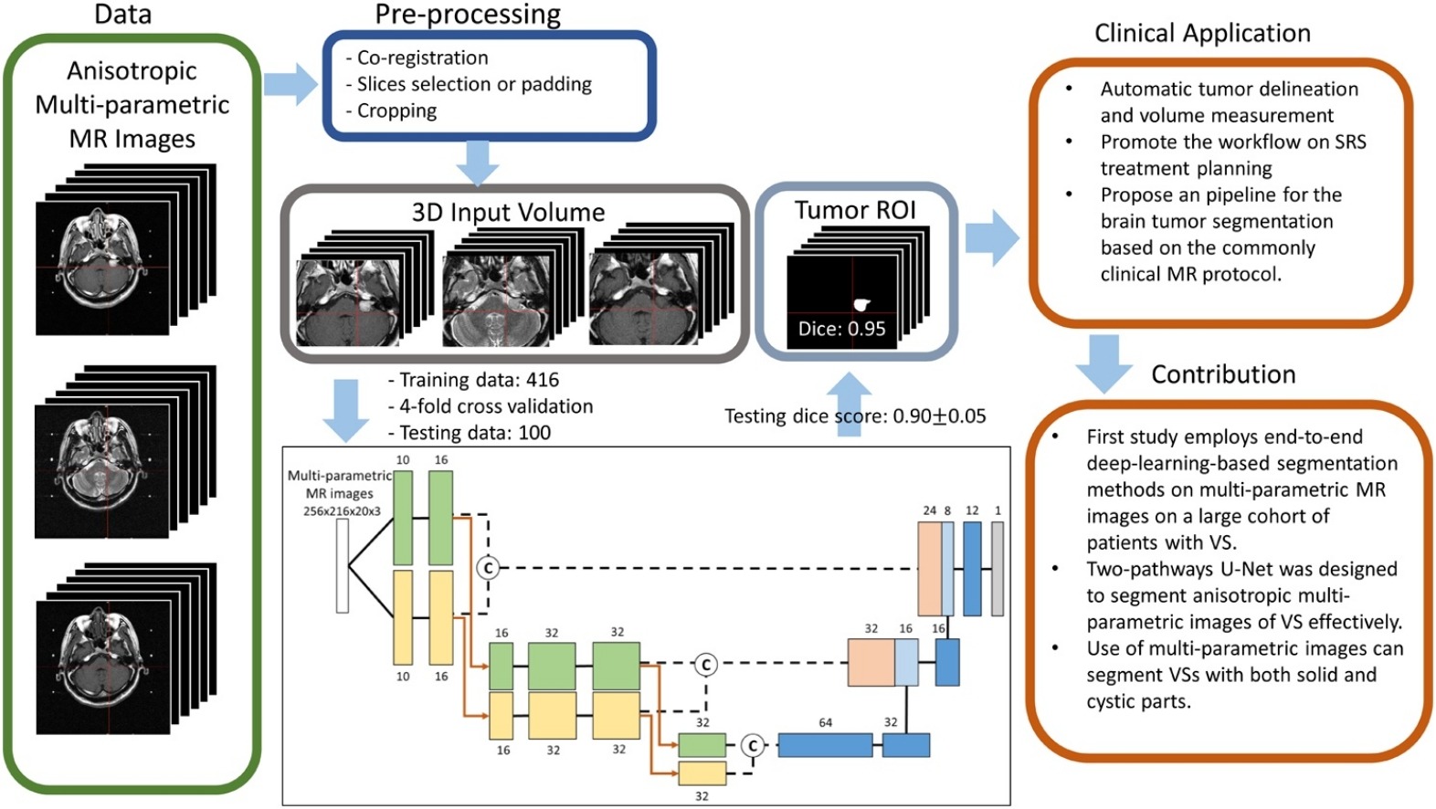
- multi-parametric MR images:T1W、T2W、T1C
- two-pathway U-Net model
- kernel 3 × 3 × 1 and 1 × 1 × 3 respectively
- to extract the in-plane and through-plane features of the anisotropic MR images
- 结论
- The proposed two-pathway U-Net model outperformed the single-pathway U-Net model when segmenting VS using anisotropic MR images.
- multi-inputs(T1、T2)outperforms single-inputs