综述
- [yolov1] Yolov1: You Only Look Once: Unified, Real-Time Object Detection
- [yolov2] Yolov2: YOLO9000: Better, Faster, Stronger
- [yolov3] Yolov3: An Incremental Improvement
- [yolov4] YOLOv4: Optimal Speed and Accuracy of Object Detection
- [poly-yolo] POLY-YOLO: HIGHER SPEED, MORE PRECISE DETECTION AND INSTANCE SEGMENTATION FOR YOLOV3
- [scaled-yolov4] Scaled-YOLOv4: Scaling Cross Stage Partial Network
- [yolov7] YOLOv7: Trainable bag-of-freebies sets new state-of-the-art for real-time object detectors
0. review
review0121:关于yolo loss
之前看keras版的yolo loss,包含分类的bce,回归的l2/mse,以及confidence的回归loss,其中conf loss被建模成单纯的0-1分类问题,用bce来实现。
事实上原版的yolo loss中,objectness是iou(pred和gt的iou),从意义上,不仅指示当前格子有无目标,还对当前的box prediction做了评估
- 回传梯度
不回传梯度
iou是通过xywh计算的,也就是说基于iou的loss做梯度回传的时候要流经box head,scaled_yolov4中把这个梯度截断,只作为一个值,对confidence进行梯度回传,
梯度不截断也没有问题,相当于对xywh再回传一个iou的loss
review1215:main features梳理
- yolov1
- yolov2
yolov3
- giou
- anchor机制
- 匹配机制:用max_iou做1v1匹配,1 in 9 (all-level),
- 回归机制:用sigmoid和exp包裹logits,作为xy和wh的偏移量
yolov4:bag-of-tricks,CSPDarknet53+PAN-SPP+yolohead,mosaic,ciou,syncBN,diou_nms
- anchor机制
- 匹配机制:不再是唯一匹配,可以跨level,只要满足iou thresh就作为positive anchor
- 回归机制
- anchor机制
scaled-yolov4:fully CSP-ized,双向FPN,scaling up出一系列模型
- CSP-block是为了scaling-up服务的,yolov3的结构一张卡batch size只能开到8,在OOM边缘试探,这篇文章将整个结构都CSP化
- 面向GPU的YOLOv4-large包含YOLOv4-P5, YOLOv4-P6, and YOLOv4-P7
- anchor机制
- 匹配机制:相比较于yolov4进一步拓展,跨level且跨网格,只要长宽比满足阈值,都作为positive anchor,同时找到gt center最近的两个邻域网格,都作为正样本
- 回归机制:重新定义了回归机制,因为跨网格,偏移量的激活区间变成[-0.5,1.5]
- loss
- loss_box:giou
- loss_obj:bce
- loss_cls:bce
1. Yolov1: You Only Look Once: Unified, Real-Time Object Detection
- 动机:
- end-to-end: 2 stages —-> 1 stage
- real-time
论点:
- past methods: complex pipelines, hard to optimize(trained separately)
- DPM use a sliding window and a classifier to evaluate an object at various locations
- R-CNN use region proposal and run classifier on the proposed boxes, then post-processing
- in this paper: you only look once at an image
- rebuild the framework as a single regression problem: single stands for you don’t have to run classifiers on each patch
- straight from image pixels to bounding box coordinates and class probabilities: straight stands for you obtain the bounding box and the classification results side by side, comparing to the previous serial pipeline
- past methods: complex pipelines, hard to optimize(trained separately)
advantages:
- fast & twice the mean average precision of other real-time systems
- CNN sees the entire image thus encodes contextual information
- generalize better
disadvantage:
- accuracy: “ it struggles to precisely localize some objects, especially small ones”
细节:
grid:
Our system divides the input image into an S × S grid.
If the center of an object falls into a grid cell, that grid cell is responsible for detecting that object.

prediction:
Each grid cell predicts B bounding boxes, confidence scores for these boxes , and C conditional class probabilities for each grid
that is an tensor
- We normalize the bounding box width and height by the image width and height so that they fall between 0 and 1.
- We parametrize the bounding box x and y coordinates to be offsets of a particular grid cell so they are also bounded between 0 and 1.
at test time:
We obtain the class-specific confidence for individual box by multiply the class probability and box confidence:
network:
the convolutional layers extract features from the image
while the fully connected layers predict the probabilities and coordinates
training:
activation:use a linear activation function for the final layer and leaky rectified linear activation all the other layers
optimization:use sum-squared error, however it does not perfectly align with the goal of maximizing average precision
* weights equally the localization error and classification error:$\lambda_{coord}$
* weights equally the grid cells containing and not-containing objects:$\lambda_{noobj}$
* weights equally the large boxes and small boxes:square roots the h&w insteand of the straight h&w
loss:pick the box predictor has the highest current IOU with the ground truth per grid cell
avoid overfitting:dropout & data augmentation
* use dropout after the first connected layer,
* introduce random scaling and translations of up to 20% of the original image size for data augmentation
* randomly adjust the exposure and saturation of the image by up to a factor of 1.5 in the HSV color space for data augmentation
inference:
multiple detections:some objects locates near the border of multiple cells and can be well localized by multiple cells. Non-maximal suppression is proved critical, adding 2- 3% in mAP.
Limitations:
- strong spatial constraints:decided by the settings of bounding boxes
softmax classification:can only have one class for each grid
“This spatial constraint lim- its the number of nearby objects that our model can pre- dict. Our model struggles with small objects that appear in groups, such as flocks of birds. “
“ It struggles to generalize to objects in new or unusual aspect ratios or configurations. “
coarse bounding box prediction:the architecture has multiple downsampling layers
the loss function treats errors the same in small bounding boxes versus large bounding boxes:
The same error has much greater effect on a small box’s IOU than a big box.
“Our main source of error is incorrect localizations. “
Comparison:
- mAP among real-time detectors and Less Than Real-Time detectors:less mAP than fast-rcnn but much faster
- error analysis between yolo and fast-rcnn:greater localization error and less background false-positive
- combination analysis:[fast-rcnn+yolo] defeats [fast-rcnn+fast-rcnn] since YOLO makes different kinds of mistakes with fast-rcnn
- generalizability:RCNN degrades more because the Selective Search is tuned for natural images, change of dataset makes the proposals get worse. YOLO degrades less because it models the size and shape of objects, change of dataset varies less at object level but more at pixel level.
2. Yolov2: YOLO9000: Better, Faster, Stronger
动机:
- run at varying sizes:offering an easy tradeoff between speed and accuracy
- recognize a wide variety of objects :jointly train on object detection and classification, so that the model can predict objects that aren’t labelled in detection data
- better performance but still fast
论点:
- Current object detection datasets are limited compared to classification datasets
- leverage the classification data to expand the scope of current detection system
- joint training algorithm making the object detectors working on both detection and classification data
- Better performance often hinges on larger networks or ensembling multiple models. However we want a more accurate detector that is still fast
- YOLOv1’s shortcomings
- more localization errors
- low recall
- Current object detection datasets are limited compared to classification datasets
要素:
better
faster
- backbone
stronger
uses labeled detection images to learn to precisely localize objects
uses classification images to increase its vocabulary and robustness
方法:
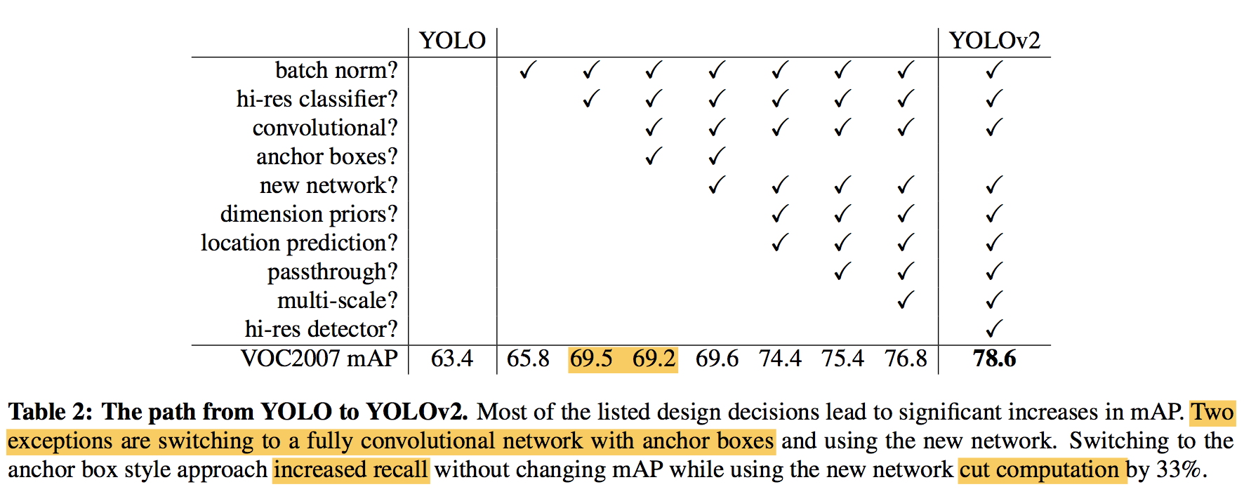
better:
batch normalization:convergence & regularization
add batch normalization on all of the convolutional layers
remove dropout from the model
high resolution classifier:pretrain a hi-res classifier
first fine tune the classification network at the full 448 × 448 resolution for 10 epochs on ImageNet
then fine tune the resulting network on detection
convolutional with anchor boxes:
YOLOv1通过网络最后的全连接层,直接预测每个grid上bounding box的坐标
而RPN基于先验框,使用最后一层卷积层,在特征图的各位置预测bounding box的offset和confidence
“Predicting offsets instead of coordinates simplifies the problem and makes it easier for the network to learn”
YOLOv2去掉了全连接层,也使用anchor box来回归bounding box
eliminate one pooling layer to make the network output have higher resolution
shrink the network input to 416416 to obtain an odd number so that there is a *single center cell in the feature map
predict class and objectness for every anchor box(offset prediction) instead of nothing(direct location&scale prediction)
dimension clustering:
what we want are priors that lead to good IOU scores, thus comes the distance metric:
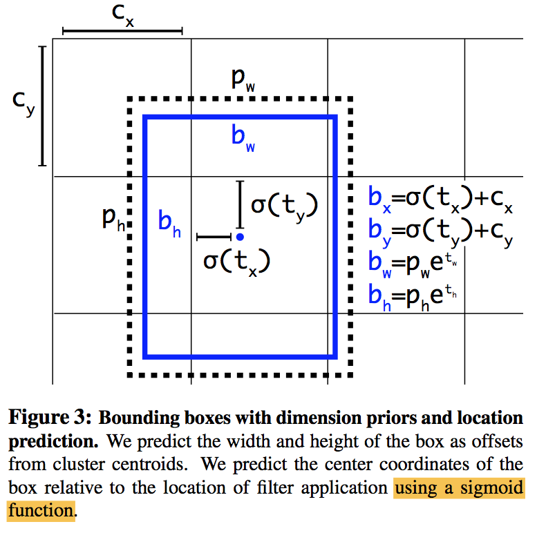
direct location prediction:
YOLOv1 encounter model instability issue for predicting the (x, y) locations for the box
RPN also takes a long time to stabilize by predicting a (tx, ty) and obtain the (x, y) center coordinates indirectly because this formulation is unconstrained so any anchor box can end up at any point in the image:
学习RPN:回归一个相对量,比盲猜回归一个绝对location(YOLOv1)更好学习
学习YOLOv1:基于cell的预测,将bounding box限定在有限区域,不是全图飞(RPN)
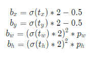
YOLOv2对每个cell,基于5个prior anchor size,预测5个bounding box,每个bounding box具有5维:
- $t_x\ \&\ t_y$用于回归bounding box的位置,通过sigmoid激活函数被限定在0-1,通过上式能够间接得到bounding box的归一化位置(相对原图)
- $t_w\ \&\ t_h$用于回归bounding box的尺度,输出应该不是0-1限定,$p_w\ \&\ p_h$是先验框的归一化尺度,通过上式能够间接得到bounding box的归一化尺度(相对原图)
- $t_o$用于回归objectness,通过sigmoid限定在0-1之间,因为$Pr(object)\ \&\ IOU(b,object)$都是0-1之间的值,IOU通过前面四个值能够求解,进而可以解耦objectness
fine-grained features:
motive:小物体的检测依赖更加细粒度的特征
cascade:Faster R-CNN and SSD both run their proposal networks at various feature maps in the network to get a range of resolutions
【QUESTION】YOLOv2 simply adds a passthrough layer from an earlier layer at 26 × 26 resolution:
latter featuremap —-> upsampling
concatenate with early featuremap
the detector runs on top of this expanded feature map
predicts a $NN(3*(4+1+80))$ tensor for each scale
multi-scale training:
模型本身不限定输入尺寸:model only uses convolutional and pooling layers thus it can be resized on the fly
- forces the network to learn to predict well across a variety of input dimensions
- the same network can predict detections at different resolutions
loss:cited from the latter yolov3 paper
- use sum of squared error loss for box coordinate(x,y,w,h):then the gradient is $y_{true} - y_{pred}$
- use logistic regression for objectness score:which should be 1 if the bounding box prior overlaps a ground truth object by more than any other bounding box prior
- if a bounding box prior is not assigned to a ground truth object it incurs no loss(coordinate&objectness)
- use binary cross-entropy loss for multilabel classification
faster:
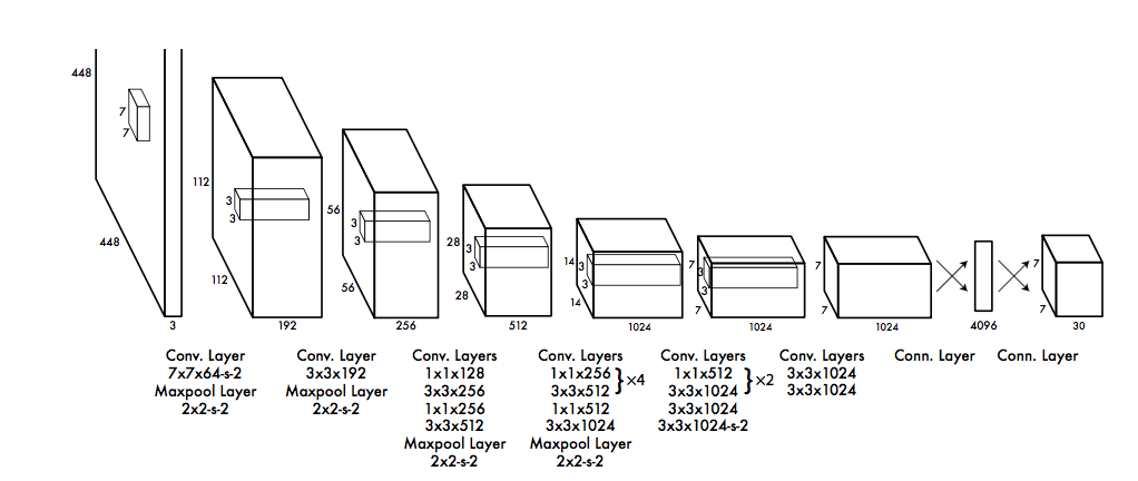
darknet-19:
YOLOv1中讨论过换VGG-16和YOLOv1使用的backbone对比,前者有map提升,但是耗时。
YOLOv2的新backbone,参数更少,而且相对于VGG16在ImageNet上精度更高。
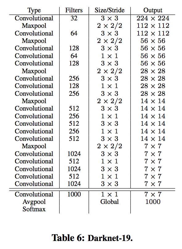
training for classification:
- first train on ImageNet using 224*224
- then fine-tuning on 448*448
training for detection:
- remove the last convolutional layer
- add on three 3 × 3 convolutional layers with 1024 filters each followed by a final 1×1 convolutional layer with the number of outputs we need for detection
- add a passthrough from the final 3 × 3 × 512 layer to the second to last convolutional layer so that our model can use fine grain features.
stronger:
jointly training:以后再填坑
- 构造标签树
- classification sample用cls loss,detection sample用detect loss
- 预测正确的classification sample给一个.3 IOU的假设值用于计算objectness loss
3. Yolov3: An Incremental Improvement
动机:
nothing like super interesting, just a bunch of small changes that make it better
方法:
bounding box prediction:
use anchor boxes and predicts offsets for each bounding box
use sum of squared error loss for training
predicts the objectness score for each bounding box using logistic regression
one ground truth coresponds to one best box and one loss
class prediction:
use binary cross-entropy loss for multilabel classification
【NEW】prediction across scales:
the detector:a few more convolutional layers following the feature map, the last of which predicts a 3-d(for 3 priors) tensor encoding bounding box, objectness, and class predictions
expanded feature map:upsampling the deeper feature map by 2X and concatenating with the former features
“With the new multi-scale predictions, YOLOv3 has better perfomance on small objects and comparatively worse performance on medium and larger size objects “
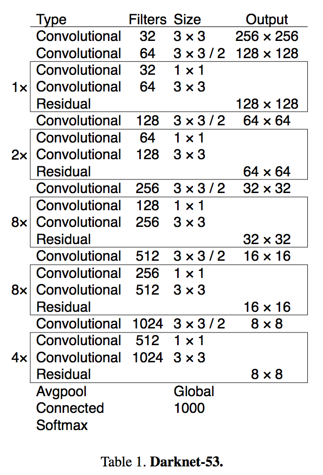
【NEW】feature extractor:
darknet-53 !
training:common skills
4. 一些补充
metrics:mAP
最早由PASCAL VOC提出,输出结果是一个ranked list,每一项包含框、confidence、class,
yolov3提到了一个“COCOs weird average mean AP metric ”
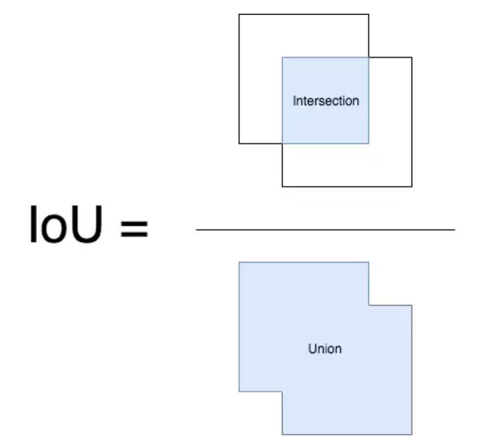
IoU:预测框与ground truth的交并比,也被称为Jaccard指数,我们通常用其来判断每个检测的正确性。PASCAL VOC数据集用0.5为阈值来判定预测框是True Positive还是False Positive,COCO数据集则建议对不同的IoU阈值进行计算。
置信度:通过改变置信度阈值,我们可以改变一个预测框是Positive还是 Negative。
precision & recall:precision = TP /(TP + FP),recall = TP/(TP + FN)。图片中我们没有预测到的每个部分都是Negative,因此计算True Negatives比较难办。但是我们只需要计算False Negatives,即我们模型所漏检的物体。
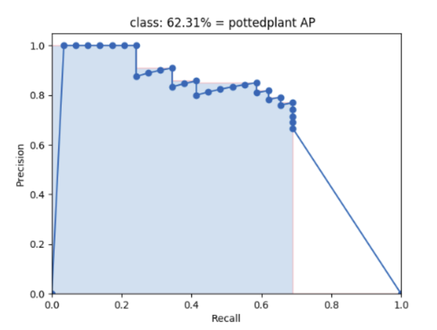
AP:不同的置信度下会得到不同的precision-recall。为了得到precision-recall曲线,首先对模型预测结果进行排序,按照各个预测值置信度降序排列。给定不同的置信度阈值,就有不同的ranked output,Recall和Precision仅在高于该rank值的预测结果中计算。这里共选择11个不同的recall([0, 0.1, …, 0.9, 1.0]),那么AP就定义为在这11个recall下precision的平均值,其可以表征整个precision-recall曲线(曲线下面积)。给定recall下的precision计算,是通过一种插值的方式:
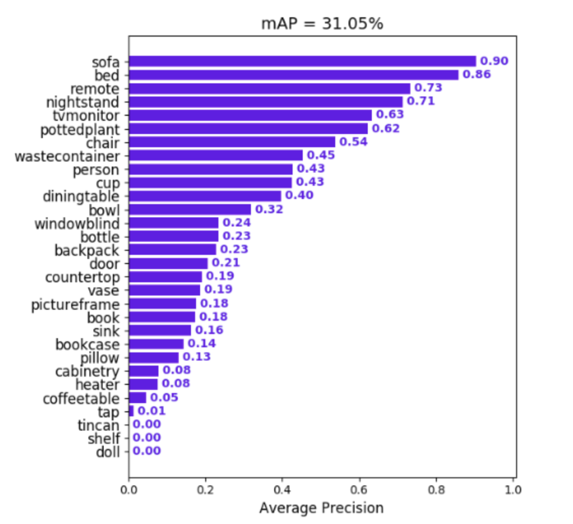
mAP:此度量指标在信息检索和目标检测领域有不同的计算方式。对于目标检测,对于各个类别,分别按照上述方式计算AP,取所有类别的AP平均值就是mAP。
eval:
- yolo_head输出:box_xy是box的中心坐标,(0~1)相对值;box_wh是box的宽高,(0~1)相对值;box_confidence是框中物体置信度;box_class_probs是类别置信度;
- yolo_correct_boxes函数:能够将box中心的相对信息转换成[y_min,x_min,y_max,x_max]的绝对值
- yolo_boxes_and_scores函数:输出网络预测的所有box
- yolo_eval函数:基于score_threshold、max_boxes两项过滤,类内NMS,得到最终输出
4. YOLOv4: Optimal Speed and Accuracy of Object Detection
动机
- Practical testing the tricks of improving CNN
- some features
- work for certain problems/dataset exclusively
- applicable to the majority of models, tasks, and datasets
- only increase the training cost [bag-of-freebies]
- only increase the inference cost by a small amount but can significantly improve the accuracy [bag-of-specials]
- Optimal Speed and Accuracy
论点
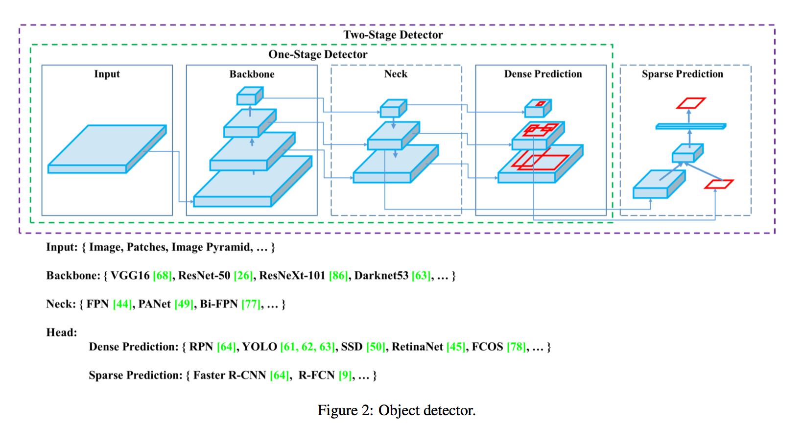
- head:
- predict classes and bounding boxes
- one-stage head
- YOLO, SSD, RetinaNet
- anchor-free:CenterNet, CornerNet, FCOS
- two-stage head
- R-CNN series
- anchor-free:RepPoints
- neck:
- collect feature maps from different stages
- FPN, PAN, BiFPN, NAS-FPN
backbone:
- pre-trained on ImageNet
- VGG, ResNet, ResNeXt, DenseNet
Bag of freebies
- data augmentation
- pixel-wise adjustments
- photometric distortions:brightness, contrast, hue, saturation, and noise
- geometric distortions:random scaling, cropping, flipping, and rotating
- object-wise
- cut:
- to image:CutOut
- to featuremaps:DropOut, DropConnect, DropBlock
- add:MixUp, CutMix, GAN
- cut:
- pixel-wise adjustments
- data imbalance for classification
- two-stage:hard example mining
- one-stage:focal loss, soft label
- bounding box regression
- MSE-regression:treat [x,y,w,h] as independent variables
- IoU loss:consider the integrity & scale invariant
- data augmentation
- Bag of specials
- enlarging receptive field:improved SPP, ASPP, RFB
- introducing attention mechanism
- channel-wise attention:SE, increase the inference time by about 10%
- point-wise attention:Spatial Attention Module (SAM), does not affect the speed of inference
- strengthening feature integration
- channel-wise level:SFAM
- point-wise level:ASFF
- scale-wise level:BiFPN
- activation function:A good activation function can make the gradient more efficiently propagated
- post-processing:各种NMS
- head:
方法
choose a backbone —- CSPDarknet53
- Higher input network size (resolution) – for detecting multiple small-sized objects
- More conv layers – for a higher receptive field to cover the increased size of input network
- More parameters – for greater capacity of a model to detect multiple objects of different sizes in a single image
add the SPP block over the CSPDarknet53
- significantly increases the receptive field
- separates out the most significant context features
- causes almost no re- duction of the network operation speed
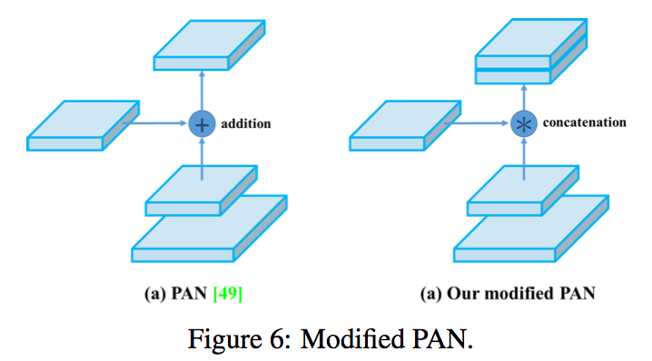
use PANet as the method of parameter aggregation
- Modified PAN
replace shortcut connection of PAN to concatenation
use YOLOv3 (anchor based) head
encoding/decoding method变了!!!
代码和issue里面有说明:https://github.com/WongKinYiu/ScaledYOLOv4/issues/90#,但是论文里没显式的说明
given pred offsets $t_x,t_y,t_w,t_h$
xy_offsets:for each grid centers
wh_ratios:for each grid anchors
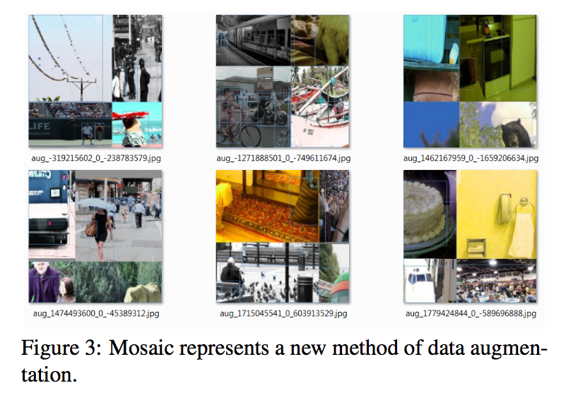
Mosaic data augmentation
- mixes 4 training images
- allows detection of objects outside their normal context
- reduces the need for a large mini-batch size
Self-Adversarial Training (SAT) data augmentation
- 1st stage alters images
- 2nd stage train on the modified images
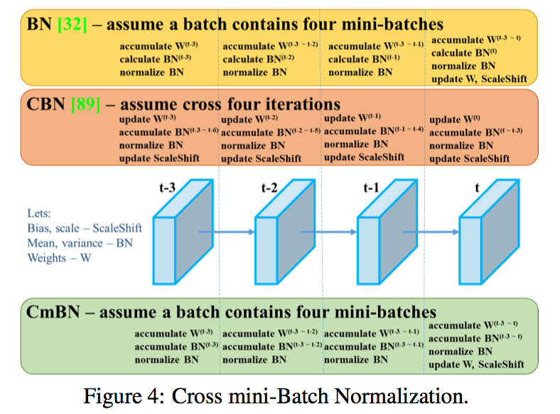
CmBN:a CBN modified version
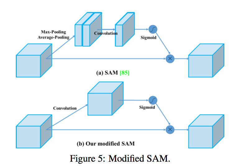
modified SAM:from spatial-wise attention to point- wise attention
- 这里的SAM for 《An Empirical Study of Spatial Attention Mechanisms in Deep Networks》 ,空间注意力机制
- 还有一篇SAM是《Sharpness-Aware Minimization for Efficiently Improving Generalization》,google的锐度感知最小化,用来提升模型泛化性能,注意区分
实验
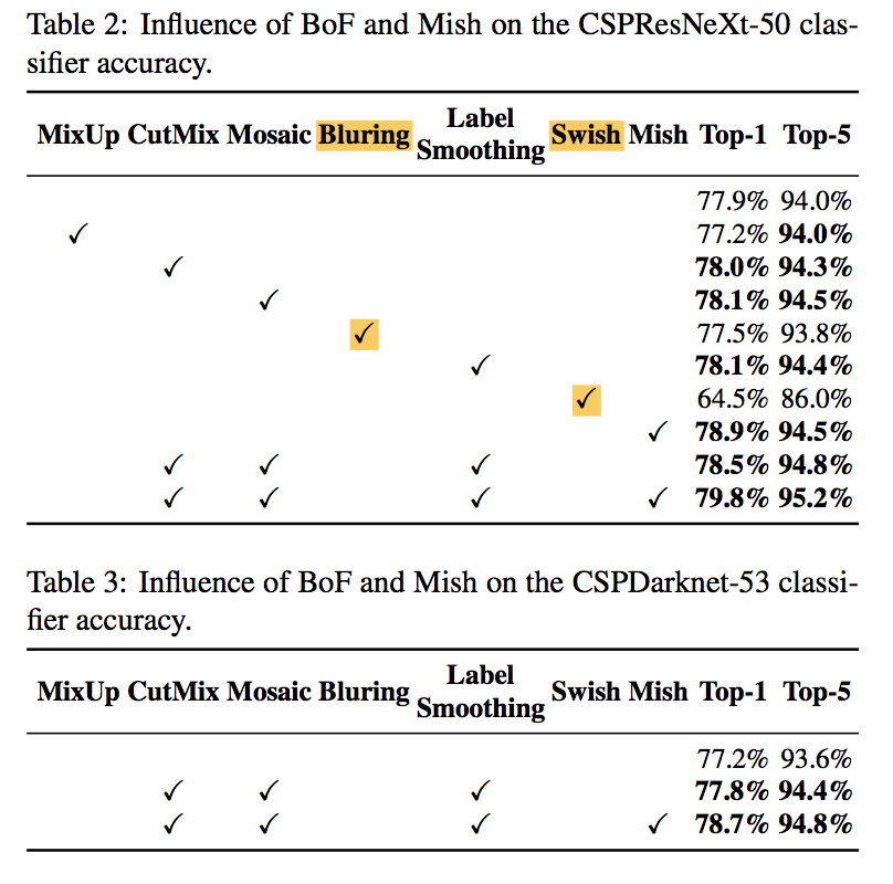
Influence of different features on Classifier training
Bluring和Swish没有提升
Influence of different features on Detector training
- IoU threshold, CmBN, Cosine annealing sheduler, CIOU有提升
POLY-YOLO: HIGHER SPEED, MORE PRECISE DETECTION AND INSTANCE SEGMENTATION FOR YOLOV3
动机
yoloV3’s weakness
- rewritten labels
- inefficient distribution of anchors
light backbone:
- stairstep upsampling
- single scale output
- to extend instance segmentation
- detect size-independent polygons defined on a polar grid
- real-time processing
论点
yolov3
- real-time
- low precision cmp with RetinaNet, EfficientDet
- low precision of the detection of big boxes
- rewriting of labels by each-other due to the coarse resolution
this paper solution:
- 解决yolo精度问题:propose a brand-new feature decoder with a single ouput tensor that goes to head with higher resolution
- 多尺度特征融合:utilize stairstep upscaling
- 实例分割:bounding polygon within a poly grid
instance segmentation
- two-stage:mask-rcnn
- one-stage:
- top-down:segmenting this object within a bounding box
- bottom-up:start with clustering pixels
- direct methods:既不需要bounding box也不需要clustered pixels,PolarMask
cmp with PolarMask
- size-independent:尺度,大小目标都能检测
- dynamic number of vertices:多边形定点可变
yolov3 issues
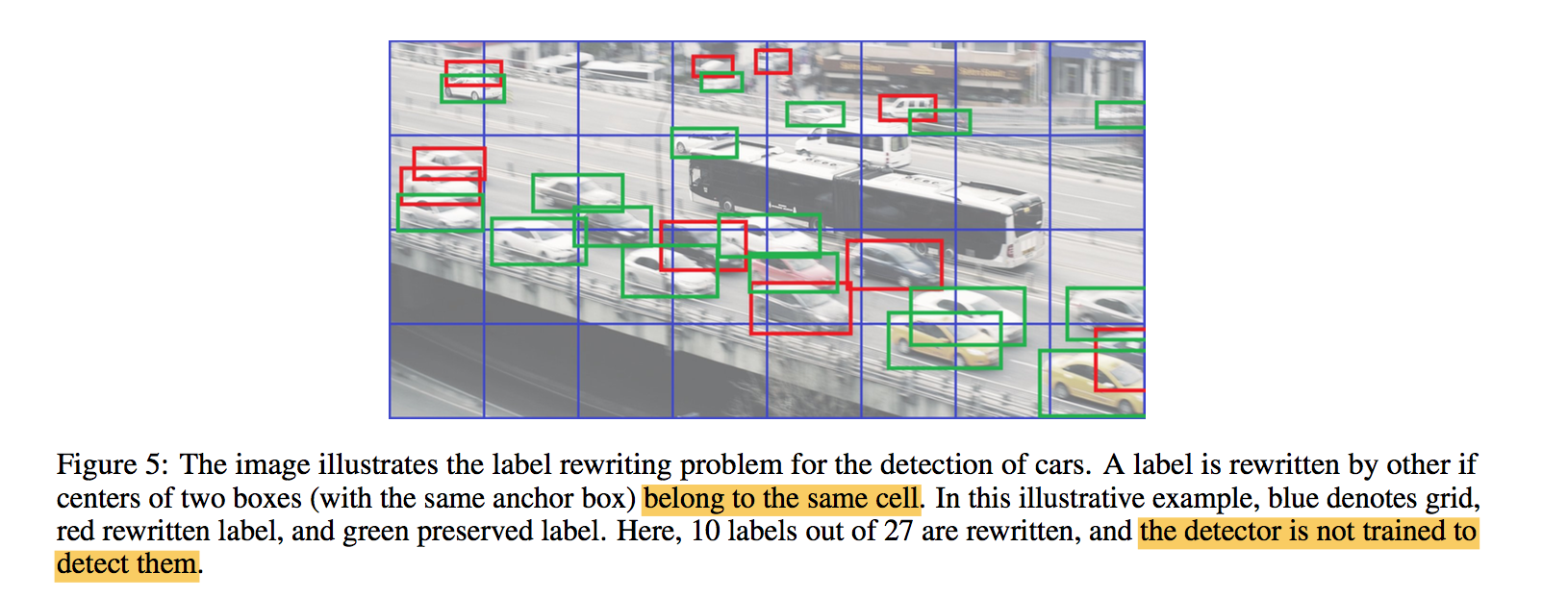
rewriting of labels:
- 两个目标如果落在同一个格子里,在一个尺度上ground truth label只会保留一个box
对越小的特征图,grid越大,这个问题越严重
imbalanced distribution of anchors across output scales
- anchor如果选的不合理,会导致特征图尺度和anchor尺度不匹配
- most of the boxes will be captured by the middle output layer and the two other layers will be underused
- 如上面车的case,大多数车的框很小,聚类出的给level0和level1的anchor shape还是很小,但是level0是稀疏grid
- 一方面,grid shape和anchor shape不匹配
- 一方面,label rewriten问题会升级
- 反过来,如果dense grid上预测大目标,会受到感受野的制约
- 一种解决方案是基于感受野首先对gt box分成三组,然后分别聚类,然后9选1
yolov3原文:YOLOv3 has relatively high $AP_{small}$ performance. However, it has comparatively worse performance on medium and larger size objects. More investigation is needed to get to the bottom of this.
- 小目标performance更好,大目标worse,主要是就是因为coarse grid上存在label rewriten问题,存在部分gt box被抑制掉了。
方法
architecture
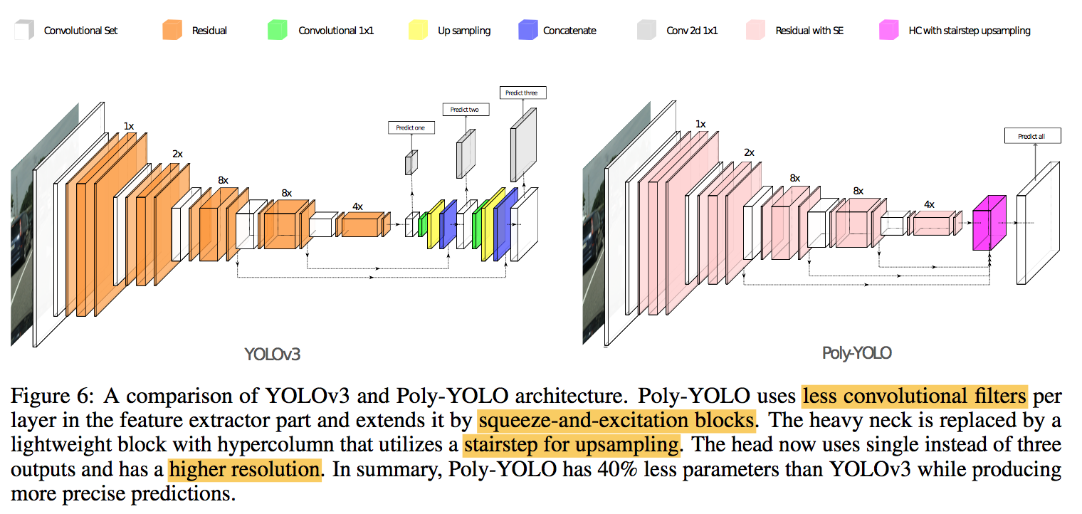
single output
higher resolution:stride4
handle all the anchors at once
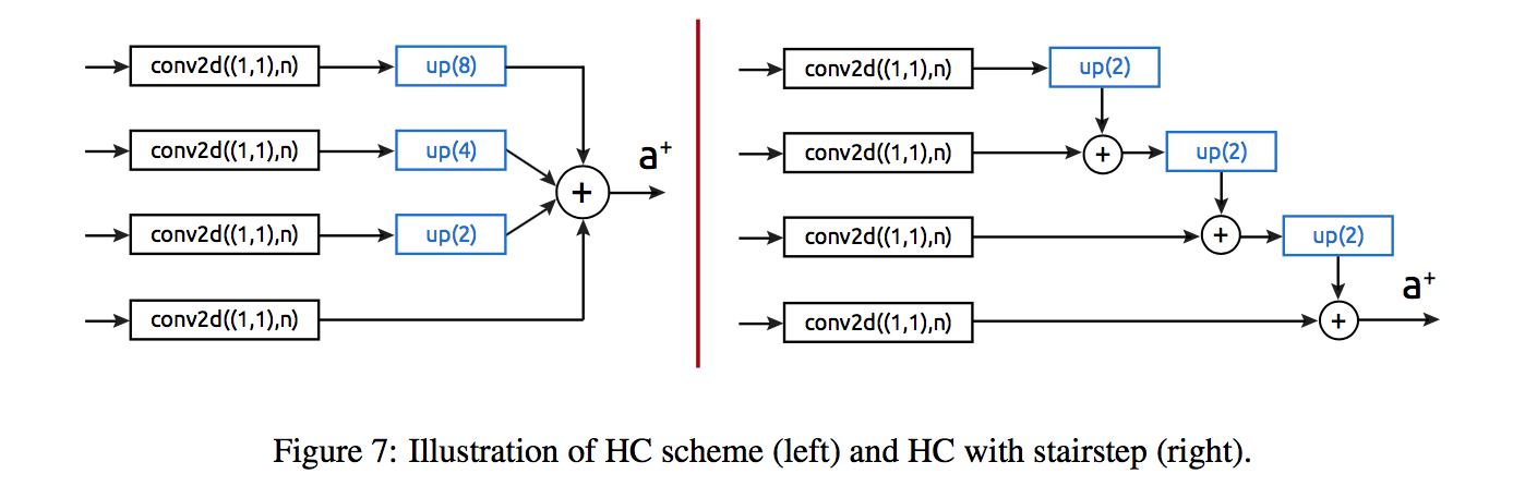
cross-scale fusion
- hypercolumn technique:add operation
stairstep interpolation:x2 x2 …
SE-blocks
- reduced the number of convolutional filters to 75% in the feature extraction phase
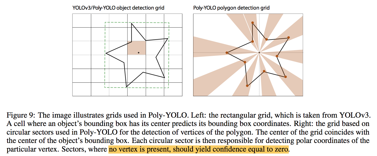
bounding polygons
- extend the box tuple:$b_i=\{b_i^{x^1},b_i^{y^1},b_i^{x^2},b_i^{y^2},V_i\}$
- The center of a bounding box is used as the origin
- polygon tuple:$v_{i,j}=\{\alpha_{i,j},\beta_{i,j},\gamma_{i,j}\}$
- polar coordinate:distance & oriented angle,相对距离(相对anchor box的对角线),相对角度(norm到[0,1])
polar cell:一定角度的扇形区域 内,如果sector内没有定点,conf=0
general shape:
- 不同尺度,形状相同的object,在polar coord下表示是一样的
- distance*anchor box的对角线,转换成绝对尺度
- bounding box的两个对角预测,负责尺度估计,polygon只负责预测形状
- sharing values should make the learning easier
mix loss
- output:a*(4+1+3*n_vmax)
- box center loss:bce
- box wh loss:l2 loss
- conf loss:bce with ignore mask
- cls loss:bce
- polygon loss:$\gamma(log(\frac{\alpha}{anchor^d})-\hat a)^2 + \gammabce(\beta,\hat{beta})+bce(\gamma, \hat \gamma)$
- auxiliary task learning:
- 任务间相互boost
- converge faster
Scaled-YOLOv4: Scaling Cross Stage Partial Network
动机
- model scaling method
- redesign yolov4 and propose yolov4-CSP
- develop scaled yolov4
- yolov4-tiny
- yolov4-large
- 没什么技术细节,就是网络结构大更新
论点
common technique changes depth & width of the backbone
recently there are NAS
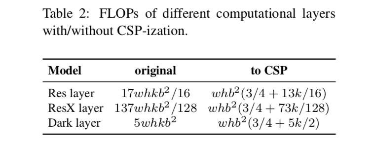
model scaling
input size、width、depth对网络计算量呈现square, linear, and square increase
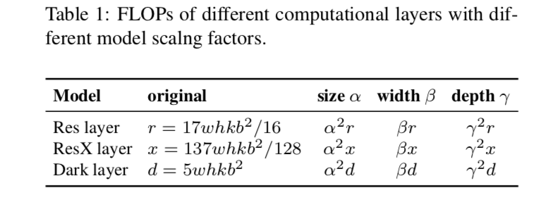
改成CSP版本以后,能够减少参数量、计算量,提高acc,缩短inference time
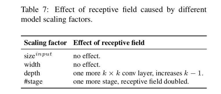
检测的准确性高度依赖reception field,RF随着depth线性增长,随着stride倍数增长,所以一般先组合调节input size和stage,然后再根据算力调整depth和width
方法
backbone:CSPDarknet53
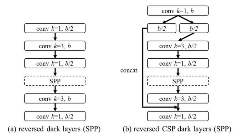
neck:CSP-PAN,减少40%计算量,SPP
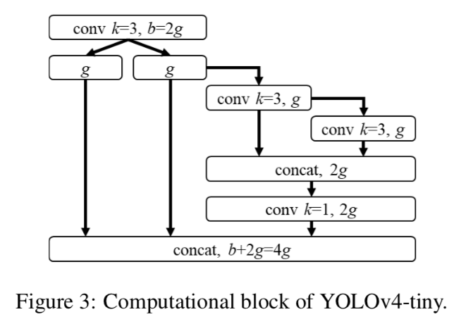
yoloV4-tiny
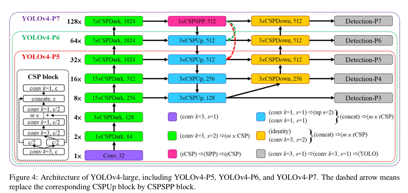
yoloV4-large:P456
补充细节
box regression
YOLOv7: Trainable bag-of-freebies sets new state-of-the-art for real-time object detectors
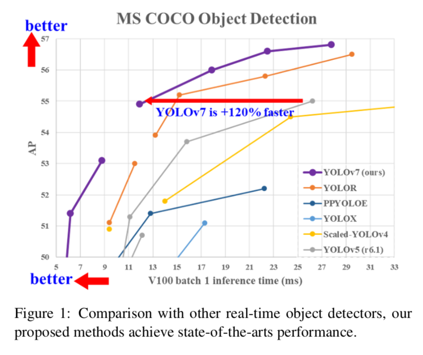
精度
- YOLOv7打败了所有real-time detectors:GPU V100上30以上FPS的模型,56.8% AP
- YOLOv7-E6打败了transformer-based (SWIN- L Cascade-Mask R-CNN)/conv-based (ConvNeXt-XL Cascade-Mask R-CNN)的两阶段模型
论点
结构上
CPU real-time detectors基本是基于MobileNet、ShuffleNet、GhostNet
GPU real-time detectors则大多数用ResNet、DarkNet、CSPNet strategy
Real-time object detectors
- 大多数基于YOLO / FCOS
- faster and stronger back
- effective feature integration
- accurate detection head
- robust loss
- a more efficient label assignment method
- a more efficient training method
- 本文关注4/5/6要素
Model re-parameterization
- merge multiple computational modules into one at inference stage
- 其实是一种模型/module层面的ensemble
- 模型层面
- ema
- k-fold ensemble
- module层面
- 线形层的合并
- 需要设计可合并的module(如非线性操作放在branch外面)
Model scaling
- 大多数NAS方法不会考虑各种factor的correlation
- darknet之类的网络实际上是compound scaling的,网络加深的同时内部block的branch就进行了同步的加宽,效果上来讲并不是孤立的增加了depth
main contribution
- 主要focus在training method上
- 优化训练进程
- 增加了training cost,但是不影响inference性能
- 所以叫trainable bag-of-freebies
- two issues & solutions
- model re-parameterization
- dynamic label assignment
- propose extent & compound scaling
- 降低40%参数量 & 50%计算量
- faster & higher acc
- 主要focus在training method上
Architecture
Extended efficient layer aggregation networks
- 考虑要素
- number of parameters
- the amount of computation
- the computational density
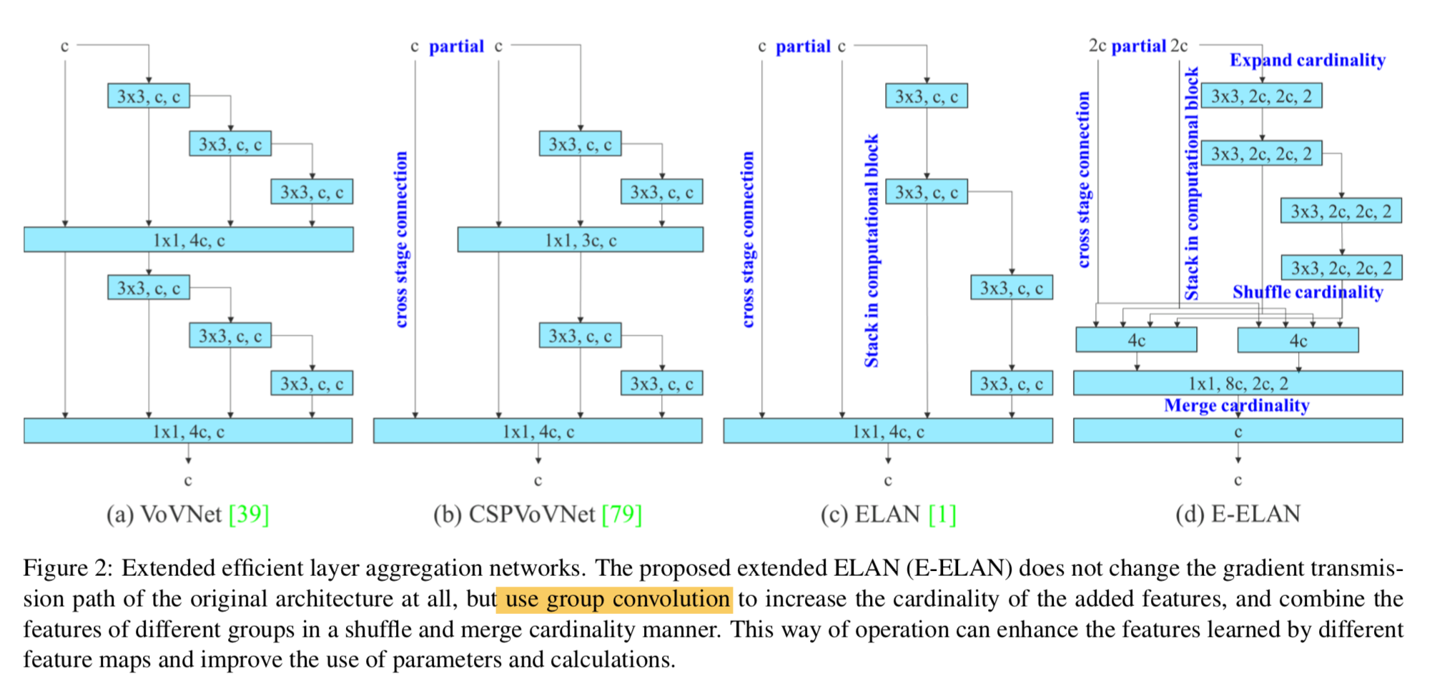
提出了Extended-ELAN
- group conv:相同计算量下,可以扩大channel(expand cardinality)
- shuffle & merge:combine the features of different groups,持续增强学习能力同时不伤害original gradient path【不太理解为啥有这个作用】
- 考虑要素
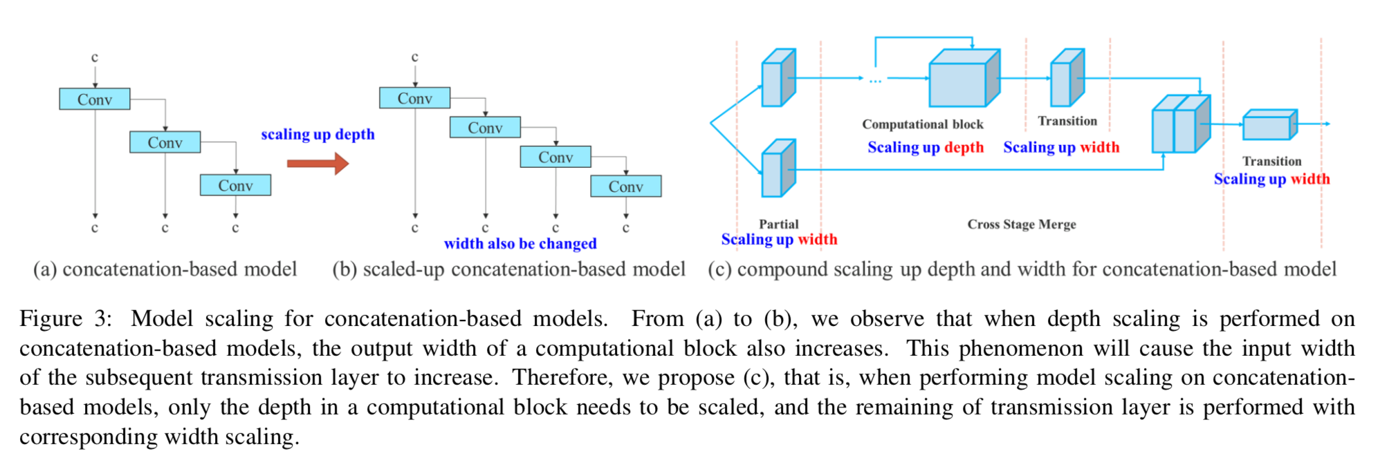
Model scaling for concatenation-based models
- 大多数讨论scaleup的网络结构,在加深时,网络内部的block的输入/输出维度不会变化,但是本文这种concatenation-based architecture,在加深时因为分支变多了,宽度也变了,因此并不能孤立探讨一个scaleup factor
compound scaling
- 在加深computation block的深度的同时,它的宽度也变了
- 因此也要同步调整其他部分的宽度
- 从而maintain the optimal structure
Trainable bag-of-freebies
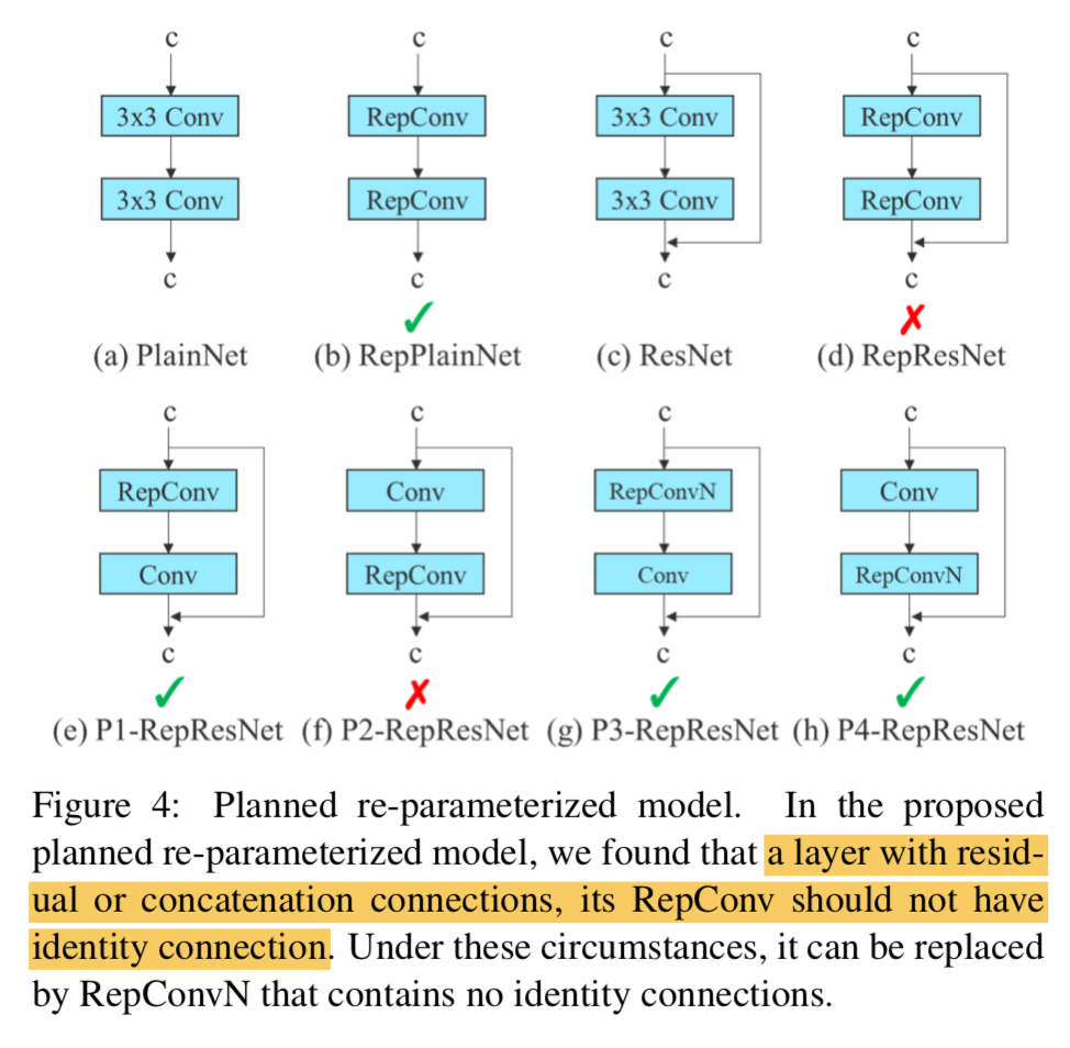
Planned re-parameterized convolution:RepConvN
受RepConv的启发,RepVGG的效果是好的,但是直接复用在resnet/densenet结构上会显著掉点
recall RepConv:inference阶段的一个3x3conv在训练阶段其实是2/3个分支(identity+1x1+3x3)
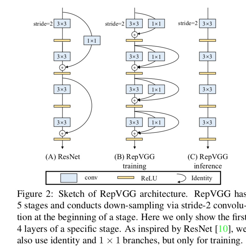
本文实验发现直接复用RepConv,它的id path会destroy the residual in ResNet/DenseNet,所以本文改良的RepConv去掉了id path(RepConvN)
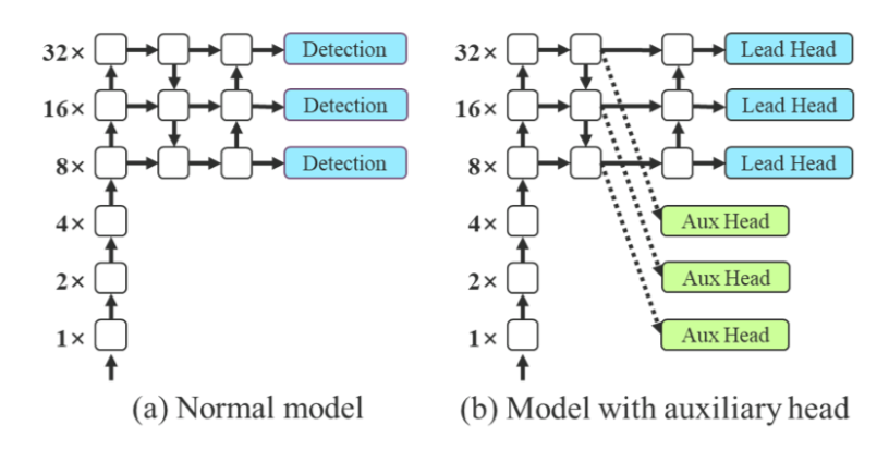
Coarse for auxiliary and fine for lead loss:label assigner
deep supervision:对中间层添加辅助分支进行loss guidance
- 保留作为最终输出的branch叫做lead head
只在训练阶段做辅助的branch叫auxiliary head
label assignment
- soft label:如用pred box和gt box的IoU作为objectness的标签,是随着网络预测结果调节标签的
- one issue:如何给每个预测头分配label,计算loss?
- 各算各的
- 用lead prediction来assign both:因为lead head的学习能力更强,生成的标签更representative一些
- this paper one step further
- 用lead prediction来assign both
- 同时生成的是coarse-to-fine的hierarchical label,to fit不同的feature level
- fine label还是上面那个lead head计算的soft label
- coarse label则allow more grids as positives,constraints放的更低了,因为让学习能力不够强的层提前学习过于精准的label,会导致后面的层学习能力恶化,但是如果前期encourage more,后期只需过滤掉低质量框就好了
- 具体实现是通过put restrictions in the decoder so that the extra coarse positive grids cannot produce soft label properly,这个fine-coarse的assign机制是在训练过程中online实现的
Other trainable bag-of-freebies
- BN:conv-bn-activation,测试阶段合并线形计算单元
- Implicit knowledge in YOLOR:测试阶段也能合并
- EMA:老ensemble了