paper2022 for SOD (salient object detection)
- SOD任务:显著目标检测,预测的是一个binary mask,无类别前景
- highly reference HED paper (Holistically-nested edge de- tection)
- https://github.com/xuebinqin/U-2-Net
U2-Net: Going Deeper with Nested U-Structure for Salient Object Detection
abstract
- propose ReSidual U-blocks (RSU)
- mixed contextual information from different scales
- deeper但是没有显著增加计算cost
- 没有用预训练backbone,直接train from scratch
- 两个版本
- u2net:176.3 MB, 30 FPS with 320x320x3 on GTX 1080Ti GPU
- u2net tiny:4.7 MB, 40 FPS
- propose ReSidual U-blocks (RSU)
introduction
use existing backbones
- 用于图像分类预训练的backbone,更多的保留的是语义信息,local details和global contrast information保留的少
- 预训练的backbone通常在第一个stem就用stride2conv+maxpooling将原图下采样到x4,但是segmentation task中high resolution map也很重要
multi-scale feature
- 3x3 conv能够很好的获取local feature
- 但是不能通过增大kernel size来获得global feature,会显著增加参数量和计算量
- this paper directly extracts multi-scale features stage by stage
- stacking UNets
- pose estimation的hourglass之类通常是sequentially stack UNets,作为cascaded refine
- this paper stack by stage
method
Residual U-blocks
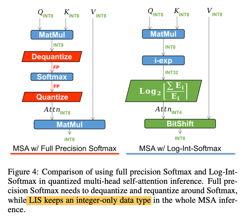
为了在high resolution的shallow layers中就学习more global information
- inception方法用了不同的dilation rate,但是memory consume
- PPM先下采样feature,然后run常规的卷积,再unsampling,但是这样恢复的feature会degrade
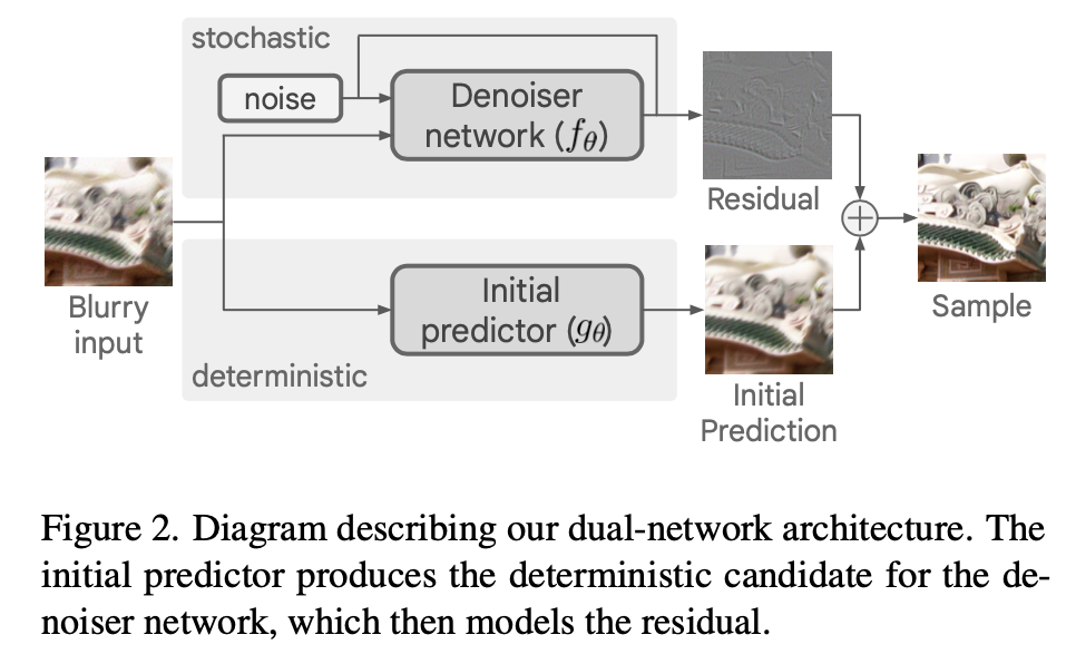
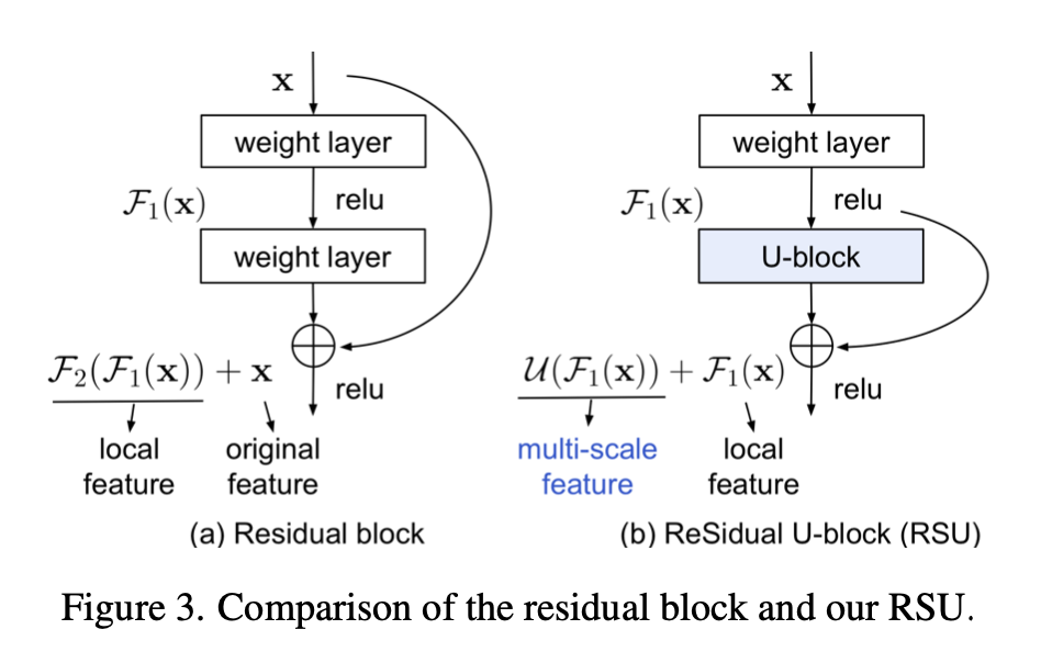
RSU three components
- an input convolution layer,用来提取local feature
- a U-Net like symmetric encoder-decoder structure with height of L,用来提取multi-scale contextual information
- larger L leads to deeper block,more pooling operations,larger reception field,richer feature
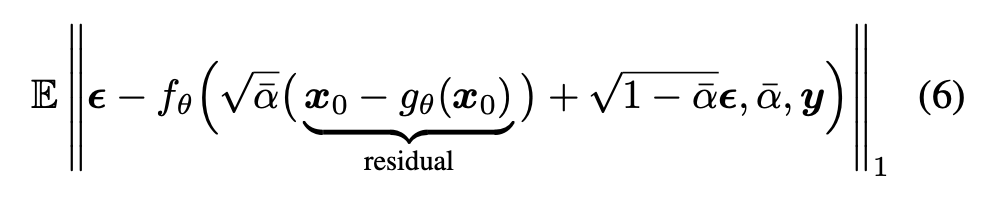
a residual connection,add local&ms feature
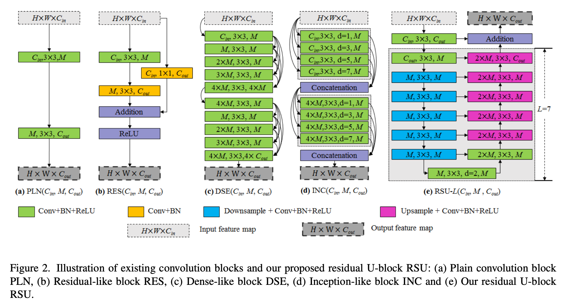
plain conv block / residual block / dense block / inception block / RSU block的对比
网络结构
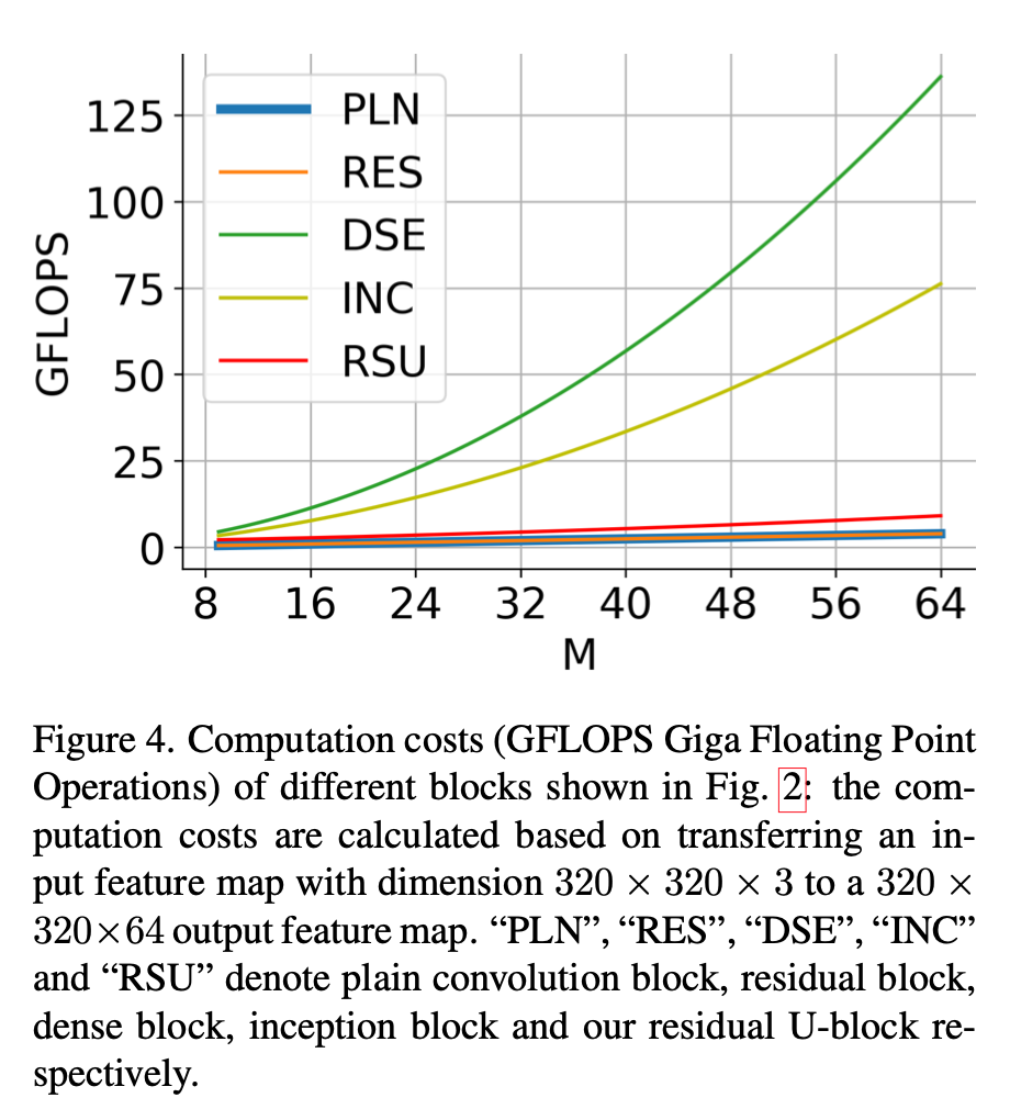
gflops对比
U2Net
overview
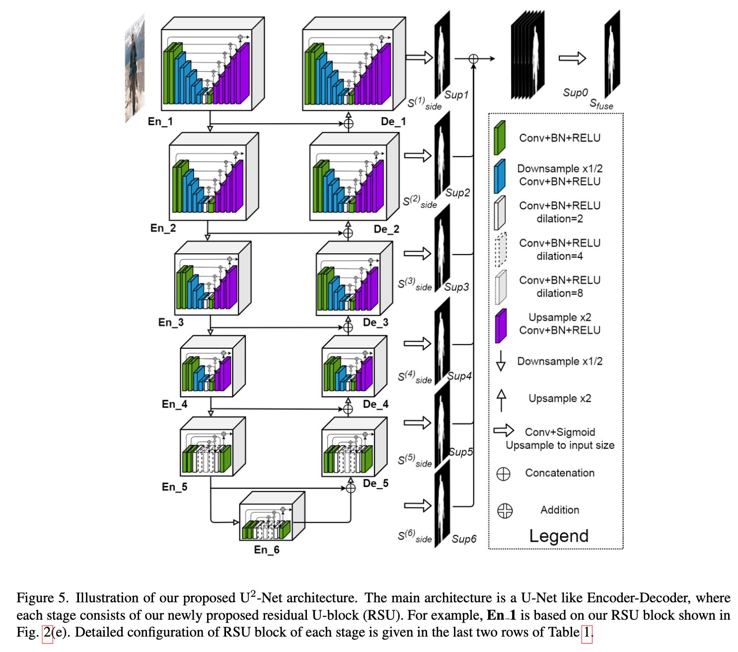
U2Net 3 parts
- a 6 stage encoder
- en1 - en4:use RSU-7, RSU-6, RSU-5 and RSU-4,7/6/5/4表示depth
- en5 - en6:RSU-4F,“F” means that the RSU is a dilated version,上/下采样都换成空洞卷积
- a 5 stage decoder
- 跟encoder镜像,输入是en-x和prev-stage unsampling的concatenation
- de5:也是空洞卷积版本的RSU-4F
- de4 - de1:RSU4-7
- a saliency map fusion module attached with the decoder stages and the last encoder stage
- side6-1:generate six side output saliency probability maps from en6,de5-1,预测头是3x3conv+sigmoid
- side fuse:upsample the logits from side6-1,concat,1x1conv+sigmoid
- a 6 stage encoder
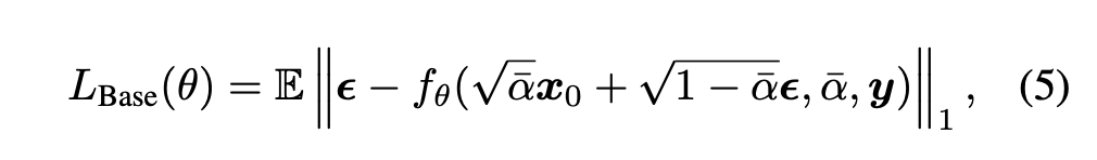
supervision
- sum loss of side6-1 & side fuse
- 每个saliency map的loss是bce
- infer time用fuse map作为final output